Trim and Fill Analysis for 'rma.uni' Objects
trimfill.RdFunction to carry out a trim and fill analysis for objects of class "rma.uni".
trimfill(x, ...)

# S3 method for class 'rma.uni'
trimfill(x, side, estimator="L0", maxiter=100, verbose=FALSE, ilim, ...)
Arguments
- x
an object of class
"rma.uni".- side
optional character string (either
"left"or"right") to specify on which side of the funnel plot the missing studies should be imputed. If left unspecified, the side is chosen within the function depending on the results of the regression test (seeregtestfor details on this test).- estimator
character string (either
"L0","R0", or"Q0") to specify the estimator for the number of missing studies (the default is"L0").- maxiter
integer to specify the maximum number of iterations for the trim and fill method (the default is
100).- verbose
logical to specify whether output should be generated on the progress of the iterative algorithm used as part of the trim and fill method (the default is
FALSE).- ilim
limits for the imputed values. If unspecified, no limits are used.
- ...
other arguments.
Details
The trim and fill method is a nonparametric (rank-based) data augmentation technique proposed by Duval and Tweedie (2000a, 2000b; see also Duval, 2005). The method can be used to estimate the number of studies missing from a meta-analysis due to suppression of the most extreme results on one side of the funnel plot. The method then augments the observed data so that the funnel plot is more symmetric and recomputes the pooled estimate based on the complete data. The trim and fill method can only be used in the context of an equal- or a random-effects model (i.e., in models without moderators). The method should not be regarded as a way of yielding a more ‘valid’ estimate of the pooled effect, but as a way of examining the sensitivity of the results to one particular selection mechanism (i.e., one particular form of publication bias).
Value
An object of class c("rma.uni.trimfill","rma.uni","rma"). The object is a list containing the same components as objects created by rma.uni, except that the data are augmented by the trim and fill method. The following components are also added:
- k0
estimated number of missing studies.
- side
either
"left"or"right", indicating on which side of the funnel plot the missing studies (if any) were imputed.- se.k0
standard error of k0.
- p.k0
p-value for the test of \(\text{H}_0\): no missing studies on the chosen side (only when
estimator="R0";NAotherwise).- yi
the observed effect size estimates plus the imputed values (if there are any).
- vi
the corresponding sampling variances
- fill
a logical vector indicating which of the values in
yiare the observed (FALSE) and the imputed (TRUE) data.
The results of the fitted model after the data augmentation are printed with the print function. Calling funnel on the object provides a funnel plot of the observed and imputed data.
Note
Three different estimators for the number of missing studies were proposed by Duval and Tweedie (2000a, 2000b). Based on these articles and Duval (2005), "R0" and "L0" are recommended. An advantage of estimator "R0" is that it provides a test of the null hypothesis that the number of missing studies (on the chosen side) is zero.
If the estimates are bounded (e.g., correlations are bounded between -1 and +1, proportions are bounded between 0 and 1), one can use the ilim argument to enforce those limits when imputing values (i.e., imputed values cannot exceed those limits then).
The model used during the trim and fill procedure is the same as used by the original model object. Hence, if an equal-effects model is passed to the function, then an equal-effects model is also used during the trim and fill procedure and the results provided are also based on an equal-effects model. This would be an ‘equal-equal’ approach. Similarly, if a random-effects model is passed to the function, then the same model is used as part of the trim and fill procedure and for the final analysis. This would be a ‘random-random’ approach. However, one can also easily fit a different model for the final analysis than was used for the trim and fill procedure. See ‘Examples’ for an illustration of an ‘equal-random’ approach.
References
Duval, S. J., & Tweedie, R. L. (2000a). Trim and fill: A simple funnel-plot-based method of testing and adjusting for publication bias in meta-analysis. Biometrics, 56(2), 455–463. https://doi.org/10.1111/j.0006-341x.2000.00455.x
Duval, S. J., & Tweedie, R. L. (2000b). A nonparametric "trim and fill" method of accounting for publication bias in meta-analysis. Journal of the American Statistical Association, 95(449), 89–98. https://doi.org/10.1080/01621459.2000.10473905
Duval, S. J. (2005). The trim and fill method. In H. R. Rothstein, A. J. Sutton, & M. Borenstein (Eds.) Publication bias in meta-analysis: Prevention, assessment, and adjustments (pp. 127–144). Chichester, England: Wiley.
Viechtbauer, W. (2010). Conducting meta-analyses in R with the metafor package. Journal of Statistical Software, 36(3), 1–48. https://doi.org/10.18637/jss.v036.i03
See also
Examples
### calculate log risk ratios and corresponding sampling variances
dat <- escalc(measure="RR", ai=tpos, bi=tneg, ci=cpos, di=cneg, data=dat.bcg)
### meta-analysis of the log risk ratios using an equal-effects model
res <- rma(yi, vi, data=dat, method="EE")
taf <- trimfill(res)
taf
#>
#> Estimated number of missing studies on the right side: 4 (SE = 2.3853)
#>
#> Equal-Effects Model (k = 17)
#>
#> I^2 (total heterogeneity / total variability): 93.91%
#> H^2 (total variability / sampling variability): 16.42
#>
#> Test for Heterogeneity:
#> Q(df = 16) = 262.7316, p-val < .0001
#>
#> Model Results:
#>
#> estimate se zval pval ci.lb ci.ub
#> -0.2910 0.0383 -7.6057 <.0001 -0.3660 -0.2160 ***
#>
#> ---
#> Signif. codes: 0 ‘***’ 0.001 ‘**’ 0.01 ‘*’ 0.05 ‘.’ 0.1 ‘ ’ 1
#>
funnel(taf, cex=1.2, legend=list(show="cis"))
 ### estimator "R0" also provides test of H0: no missing studies (on the chosen side)
taf <- trimfill(res, estimator="R0")
taf
#>
#> Estimated number of missing studies on the right side: 4 (SE = 3.1623)
#> Test of H0: no missing studies on the right side: p-val = 0.0312
#>
#> Equal-Effects Model (k = 17)
#>
#> I^2 (total heterogeneity / total variability): 93.91%
#> H^2 (total variability / sampling variability): 16.42
#>
#> Test for Heterogeneity:
#> Q(df = 16) = 262.7316, p-val < .0001
#>
#> Model Results:
#>
#> estimate se zval pval ci.lb ci.ub
#> -0.2910 0.0383 -7.6057 <.0001 -0.3660 -0.2160 ***
#>
#> ---
#> Signif. codes: 0 ‘***’ 0.001 ‘**’ 0.01 ‘*’ 0.05 ‘.’ 0.1 ‘ ’ 1
#>
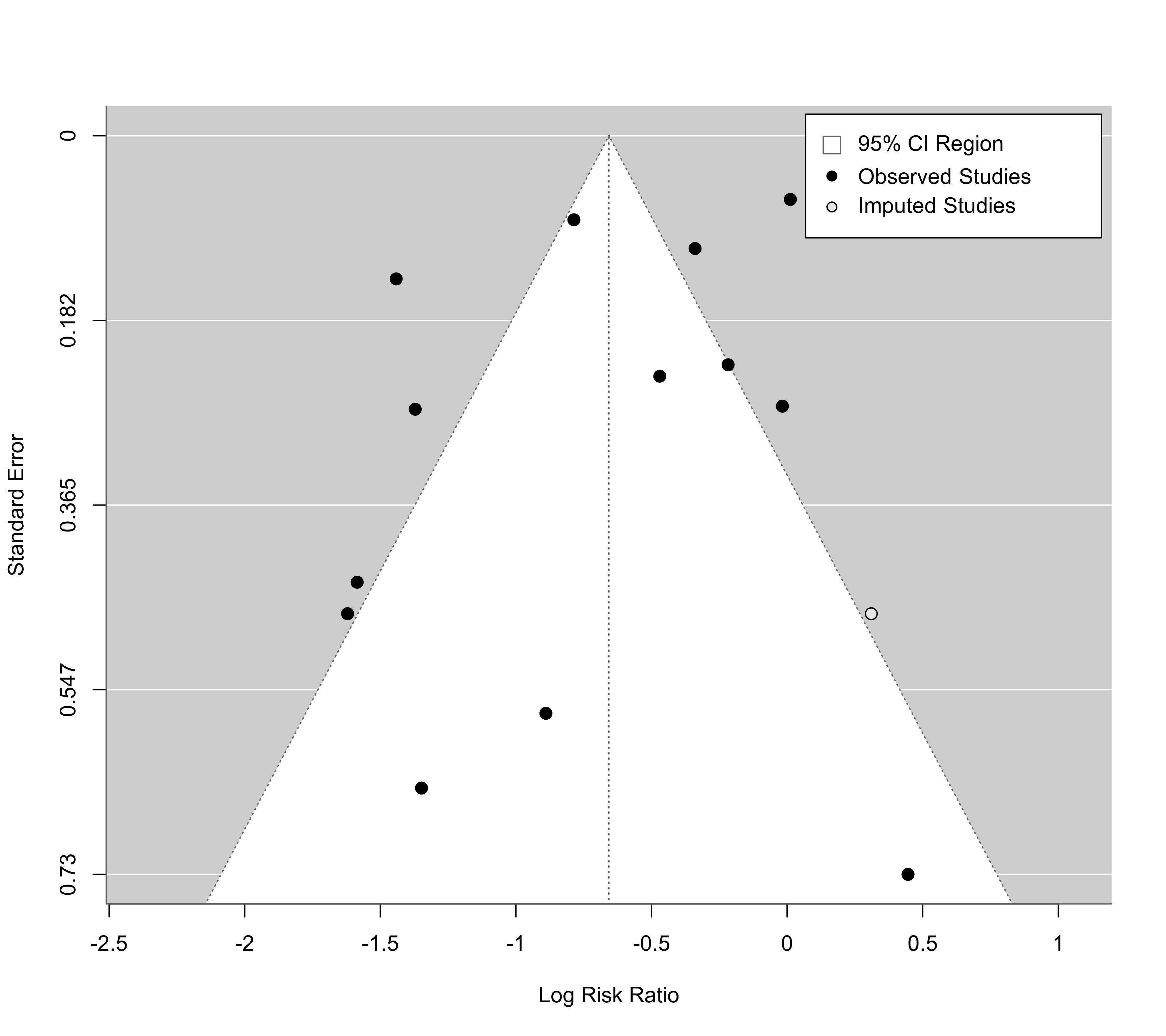
### meta-analysis of the log risk ratios using a random-effects model
res <- rma(yi, vi, data=dat)
taf <- trimfill(res)
taf
#>
#> Estimated number of missing studies on the right side: 1 (SE = 2.4528)
#>
#> Random-Effects Model (k = 14; tau^2 estimator: REML)
#>
#> tau^2 (estimated amount of total heterogeneity): 0.3313 (SE = 0.1701)
#> tau (square root of estimated tau^2 value): 0.5756
#> I^2 (total heterogeneity / total variability): 92.14%
#> H^2 (total variability / sampling variability): 12.72
#>
#> Test for Heterogeneity:
#> Q(df = 13) = 154.6750, p-val < .0001
#>
#> Model Results:
#>
#> estimate se zval pval ci.lb ci.ub
#> -0.6571 0.1785 -3.6805 0.0002 -1.0070 -0.3072 ***
#>
#> ---
#> Signif. codes: 0 ‘***’ 0.001 ‘**’ 0.01 ‘*’ 0.05 ‘.’ 0.1 ‘ ’ 1
#>
funnel(taf, cex=1.2, legend=list(show="cis"))
### estimator "R0" also provides test of H0: no missing studies (on the chosen side)
taf <- trimfill(res, estimator="R0")
taf
#>
#> Estimated number of missing studies on the right side: 4 (SE = 3.1623)
#> Test of H0: no missing studies on the right side: p-val = 0.0312
#>
#> Equal-Effects Model (k = 17)
#>
#> I^2 (total heterogeneity / total variability): 93.91%
#> H^2 (total variability / sampling variability): 16.42
#>
#> Test for Heterogeneity:
#> Q(df = 16) = 262.7316, p-val < .0001
#>
#> Model Results:
#>
#> estimate se zval pval ci.lb ci.ub
#> -0.2910 0.0383 -7.6057 <.0001 -0.3660 -0.2160 ***
#>
#> ---
#> Signif. codes: 0 ‘***’ 0.001 ‘**’ 0.01 ‘*’ 0.05 ‘.’ 0.1 ‘ ’ 1
#>
### meta-analysis of the log risk ratios using a random-effects model
res <- rma(yi, vi, data=dat)
taf <- trimfill(res)
taf
#>
#> Estimated number of missing studies on the right side: 1 (SE = 2.4528)
#>
#> Random-Effects Model (k = 14; tau^2 estimator: REML)
#>
#> tau^2 (estimated amount of total heterogeneity): 0.3313 (SE = 0.1701)
#> tau (square root of estimated tau^2 value): 0.5756
#> I^2 (total heterogeneity / total variability): 92.14%
#> H^2 (total variability / sampling variability): 12.72
#>
#> Test for Heterogeneity:
#> Q(df = 13) = 154.6750, p-val < .0001
#>
#> Model Results:
#>
#> estimate se zval pval ci.lb ci.ub
#> -0.6571 0.1785 -3.6805 0.0002 -1.0070 -0.3072 ***
#>
#> ---
#> Signif. codes: 0 ‘***’ 0.001 ‘**’ 0.01 ‘*’ 0.05 ‘.’ 0.1 ‘ ’ 1
#>
funnel(taf, cex=1.2, legend=list(show="cis"))
 ### the examples above are equal-equal and random-random approaches
### illustration of an equal-random approach
res <- rma(yi, vi, data=dat, method="EE")
taf <- trimfill(res)
filled <- data.frame(yi = taf$yi, vi = taf$vi, fill = taf$fill)
filled
#> yi vi fill
#> 1 -0.88931133 0.325584765 FALSE
#> 2 -1.58538866 0.194581121 FALSE
#> 3 -1.34807315 0.415367965 FALSE
#> 4 -1.44155119 0.020010032 FALSE
#> 5 -0.21754732 0.051210172 FALSE
#> 6 -0.78611559 0.006905618 FALSE
#> 7 -1.62089822 0.223017248 FALSE
#> 8 0.01195233 0.003961579 FALSE
#> 9 -0.46941765 0.056434210 FALSE
#> 10 -1.37134480 0.073024794 FALSE
#> 11 -0.33935883 0.012412214 FALSE
#> 12 0.44591340 0.532505845 FALSE
#> 13 -0.01731395 0.071404660 FALSE
#> 14 0.78929282 0.073024794 TRUE
#> 15 0.85949921 0.020010032 TRUE
#> 16 1.00333667 0.194581121 TRUE
#> 17 1.03884624 0.223017248 TRUE
rma(yi, vi, data=filled)
#>
#> Random-Effects Model (k = 17; tau^2 estimator: REML)
#>
#> tau^2 (estimated amount of total heterogeneity): 0.7164 (SE = 0.2944)
#> tau (square root of estimated tau^2 value): 0.8464
#> I^2 (total heterogeneity / total variability): 96.03%
#> H^2 (total variability / sampling variability): 25.19
#>
#> Test for Heterogeneity:
#> Q(df = 16) = 262.7316, p-val < .0001
#>
#> Model Results:
#>
#> estimate se zval pval ci.lb ci.ub
#> -0.3422 0.2223 -1.5392 0.1237 -0.7780 0.0936
#>
#> ---
#> Signif. codes: 0 ‘***’ 0.001 ‘**’ 0.01 ‘*’ 0.05 ‘.’ 0.1 ‘ ’ 1
#>
### the examples above are equal-equal and random-random approaches
### illustration of an equal-random approach
res <- rma(yi, vi, data=dat, method="EE")
taf <- trimfill(res)
filled <- data.frame(yi = taf$yi, vi = taf$vi, fill = taf$fill)
filled
#> yi vi fill
#> 1 -0.88931133 0.325584765 FALSE
#> 2 -1.58538866 0.194581121 FALSE
#> 3 -1.34807315 0.415367965 FALSE
#> 4 -1.44155119 0.020010032 FALSE
#> 5 -0.21754732 0.051210172 FALSE
#> 6 -0.78611559 0.006905618 FALSE
#> 7 -1.62089822 0.223017248 FALSE
#> 8 0.01195233 0.003961579 FALSE
#> 9 -0.46941765 0.056434210 FALSE
#> 10 -1.37134480 0.073024794 FALSE
#> 11 -0.33935883 0.012412214 FALSE
#> 12 0.44591340 0.532505845 FALSE
#> 13 -0.01731395 0.071404660 FALSE
#> 14 0.78929282 0.073024794 TRUE
#> 15 0.85949921 0.020010032 TRUE
#> 16 1.00333667 0.194581121 TRUE
#> 17 1.03884624 0.223017248 TRUE
rma(yi, vi, data=filled)
#>
#> Random-Effects Model (k = 17; tau^2 estimator: REML)
#>
#> tau^2 (estimated amount of total heterogeneity): 0.7164 (SE = 0.2944)
#> tau (square root of estimated tau^2 value): 0.8464
#> I^2 (total heterogeneity / total variability): 96.03%
#> H^2 (total variability / sampling variability): 25.19
#>
#> Test for Heterogeneity:
#> Q(df = 16) = 262.7316, p-val < .0001
#>
#> Model Results:
#>
#> estimate se zval pval ci.lb ci.ub
#> -0.3422 0.2223 -1.5392 0.1237 -0.7780 0.0936
#>
#> ---
#> Signif. codes: 0 ‘***’ 0.001 ‘**’ 0.01 ‘*’ 0.05 ‘.’ 0.1 ‘ ’ 1
#>