Funnel Plots
funnel.RdFunction to create funnel plots.
funnel(x, ...)

# S3 method for class 'rma'
funnel(x, yaxis="sei",
       xlim, ylim, xlab, ylab, slab,
       steps=5, at, atransf, targs, digits, level=x$level,
       addtau2=FALSE, type="rstandard",
       back, shade, hlines,
       refline, lty=3, pch, pch.fill, col, bg,
       label=FALSE, offset=0.4, legend=FALSE, ...)

# Default S3 method
funnel(x, vi, sei, ni, subset, yaxis="sei",
       xlim, ylim, xlab, ylab, slab,
       steps=5, at, atransf, targs, digits, level=95,
       back, shade, hlines,
       refline=0, lty=3, pch, col, bg,
       label=FALSE, offset=0.4, legend=FALSE, ...)
Arguments
- x
an object of class
"rma"or a vector with the effect size estimates.- vi
vector with the corresponding sampling variances (needed if
xis a vector with estimates.- sei
vector with the corresponding standard errors (note: only one of the two,
viorsei, needs to be specified).- ni
vector with the corresponding sample sizes. Only relevant when passing a vector via
x.- subset
optional (logical or numeric) vector to specify the subset of studies that should be included in the plot. Only relevant when passing a vector via
x.- yaxis
either
"sei","vi","seinv","vinv","ni","ninv","sqrtni","sqrtninv","lni", or"wi"to specify what values should be placed on the y-axis. See ‘Details’.- xlim
x-axis limits. If unspecified, the function sets the x-axis limits to some sensible values.
- ylim
y-axis limits. If unspecified, the function sets the y-axis limits to some sensible values.
- xlab
title for the x-axis. If unspecified, the function sets an appropriate axis title.
- ylab
title for the y-axis. If unspecified, the function sets an appropriate axis title.
- slab
optional vector with labels for the \(k\) studies. If unspecified, the function tries to extract study labels from
x.- steps
the number of tick marks for the y-axis (the default is 5).
- at
position of the x-axis tick marks and corresponding labels. If unspecified, the function sets the tick mark positions/labels to some sensible values.
- atransf
optional argument to specify a function to transform the x-axis labels (e.g.,
atransf=exp; see also transf). If unspecified, no transformation is used.- targs
optional arguments needed by the function specified via
atransf.- digits
optional integer to specify the number of decimal places to which the tick mark labels of the x- and y-axis should be rounded. Can also be a vector of two integers, the first to specify the number of decimal places for the x-axis, the second for the y-axis labels (e.g.,
digits=c(2,3)). If unspecified, the function tries to set the argument to some sensible values.- level
numeric value between 0 and 100 to specify the level of the pseudo confidence interval region (see here for details). For
"rma"objects, the default is to take the value from the object. May also be a vector of values to obtain multiple regions (for contour-enhanced funnel plots). See ‘Examples’.- addtau2
logical to specify whether the amount of heterogeneity should be accounted for when drawing the pseudo confidence interval region (the default is
FALSE). Ignored whenxis a meta-regression model and residuals are plotted. See ‘Details’.- type
either
"rstandard"(default) or"rstudent"to specify whether the usual or deleted residuals should be used in creating the funnel plot whenxis a meta-regression model. See ‘Details’.- back
optional character string to specify the color of the plotting region background.
- shade
optional character string to specify the color of the pseudo confidence interval region. When
levelis a vector of values, different shading colors can be specified for each region.- hlines
optional character string to specify the color of the horizontal reference lines.
- refline
numeric value to specify the location of the vertical ‘reference’ line and where the pseudo confidence interval should be centered. If unspecified, the reference line is drawn at the pooled estimate from an equal- or random-effects model and at zero for meta-regression models (in which case the residuals are plotted) or when directly passing a set of estimates to the function.
- lty
line type for the pseudo confidence interval region and the reference line. The default is to draw dotted lines (see
parfor other options). Can also be a vector to specify the two line types separately.- pch
plotting symbol to use for the estimates. By default, a filled circle is used. Can also be a vector of values. See
pointsfor other options.- pch.fill
plotting symbol to use for estimates filled in by the trim and fill method. By default, an open circle is used. Only relevant when plotting an object created by the
trimfillfunction.- col
optional character string to specify the (border) color of the points. Can also be a vector.
- bg
optional character string to specify the background color of open plot symbols. Can also be a vector.
- label
argument to control the labeling of the points (the default is
FALSE). See ‘Details’.- offset
argument to control the distance between the points and the corresponding labels.
- legend
logical to specify whether a legend should be added to the plot (the default is
FALSE). See ‘Details’.- ...
other arguments.
Details
For equal- and random-effects models (i.e., models not involving moderators), the plot shows the effect size estimates on the x-axis against the corresponding standard errors (i.e., the square root of the sampling variances) on the y-axis. A vertical line indicates the pooled estimate based on the model (or at the value specified via the refline argument). A pseudo confidence interval region is drawn around this value with bounds equal to \(\pm 1.96 \text{SE}\) (assuming level=95), where \(\text{SE}\) is the standard error value from the y-axis. If addtau2=TRUE (only for models of class "rma.uni"), then the bounds of the pseudo confidence interval region are equal to \(\pm 1.96 \sqrt{\text{SE}^2 + \hat{\tau}^2}\), where \(\hat{\tau}^2\) is the amount of heterogeneity as estimated by the model.
The level argument can be an entire vector to highlight multiple pseudo confidence interval regions in the plot. The shade argument can be used to specify the corresponding colors (if unspecified, default colors are chosen). This way, one draw contour-enhanced funnel plots (Peters et al., 2008).
For (mixed-effects) meta-regression models (i.e., models involving moderators), the plot shows the residuals on the x-axis against their corresponding standard errors. Either the usual or deleted residuals can be used for that purpose (set via the type argument). See residuals for more details on the different types of residuals.
With the atransf argument, the labels on the x-axis can be transformed with some suitable function. For example, when plotting log odds ratios, one could use transf=exp to obtain a funnel plot with the values on the x-axis corresponding to the odds ratios. See also transf for some other useful transformation functions in the context of a meta-analysis.
Instead of placing the standard errors on the y-axis, several other options are available by setting the yaxis argument to:
yaxis="vi"for the sampling variances,yaxis="seinv"for the inverse of the standard errors,yaxis="vinv"for the inverse of the sampling variances,yaxis="ni"for the sample sizes,yaxis="ninv"for the inverse of the sample sizes,yaxis="sqrtni"for the square root of the sample sizes,yaxis="sqrtninv"for the inverse square root of the sample sizes,yaxis="lni"for the log of the sample sizes,yaxis="wi"for the weights.
However, only when yaxis="sei" (the default) will the pseudo confidence region have the expected (upside-down) funnel shape with straight lines. Also, when placing (a function of) the sample sizes or the weights on the y-axis, then the pseudo confidence region cannot be drawn. See Sterne and Egger (2001) for more details on the choice of the y-axis.
If the object passed to the function comes from the trimfill function, the studies that are filled in by the trim and fill method are also added to the funnel plot. The symbol to use for plotting the filled in studies can be specified via the pch.fill argument. Arguments col and bg can then be of length 2 to specify the (border) color and background color of the observed and filled in studies.
One can also directly pass a vector with estimates (via x) and the corresponding sampling variances (via vi), standard errors (via sei), and/or sample sizes (via ni) to the function. By default, the vertical reference line is then drawn at zero.
The arguments back, shade, and hlines can be set to NULL to suppress the shading and the horizontal reference line. One can also suppress the funnel by setting refline to NULL. Using refline2, one can also add a second reference line with a funnel to the plot (see ‘Examples’).
With the label argument, one can control whether points in the plot will be labeled. If label="all" (or label=TRUE), all points in the plot will be labeled. If label="out", points falling outside of the pseudo confidence region will be labeled. Finally, one can also set this argument to a numeric value (between 1 and \(k\)) to specify how many of the most extreme points should be labeled (e.g., with label=1 only the most extreme point are labeled, while with label=3, the most extreme, and the second and third most extreme points are labeled). With the offset argument, one can adjust the distance between the labels and the corresponding points.
By setting the legend argument to TRUE, a legend is added to the plot. One can also use a keyword for this argument to specify the position of the legend (e.g., legend="topright"; see legend for options). Finally, this argument can also be a list, with elements x, y, inset, bty, and bg, which are passed on to the corresponding arguments of the legend function for even more control (elements not specified are set to defaults). The list can also include elements studies (a logical to specify whether to include ‘Studies’ in the legend; default is TRUE) and show (either "pvals" to show the p-values corresponding to the shade regions, "cis" to show the confidence interval levels corresponding to the shade regions, or NA to show neither; default is "pvals").
Note
Placing (a function of) the sample sizes on the y-axis (i.e., using yaxis="ni", yaxis="ninv", yaxis="sqrtni", yaxis="sqrtninv", or yaxis="lni") is only possible when information about the sample sizes is actually stored within the object passed to the funnel function. That should automatically be the case when the estimates were computed with the escalc function or when the estimates were computed within the model fitting function. On the other hand, this will not be the case when rma.uni was used together with the yi and vi arguments and the yi and vi values were not computed with escalc. In that case, it is still possible to pass information about the sample sizes to the rma.uni function (e.g., use rma.uni(yi, vi, ni=ni, data=dat), where data frame dat includes a variable called ni with the sample sizes).
When using unweighted estimation, using yaxis="wi" will place all points on a horizontal line. When directly passing a vector with the estimates to the function, yaxis="wi" is equivalent to yaxis="vinv", except that the weights are expressed in percent.
For argument slab and when specifying vectors for arguments pch, col, and/or bg and when x is an object of class "rma", the variables specified are assumed to be of the same length as the data passed to the model fitting function (and if the data argument was used in the original model fit, then the variables will be searched for within this data frame first). Any subsetting and removal of studies with missing values is automatically applied to the variables specified via these arguments.
Value
A data frame with components:
- x
the x-axis coordinates of the points that were plotted.
- y
the y-axis coordinates of the points that were plotted.
- slab
the study labels.
Note that the data frame is returned invisibly.
References
Light, R. J., & Pillemer, D. B. (1984). Summing up: The science of reviewing research. Cambridge, MA: Harvard University Press.
Peters, J. L., Sutton, A. J., Jones, D. R., Abrams, K. R., & Rushton, L. (2008). Contour-enhanced meta-analysis funnel plots help distinguish publication bias from other causes of asymmetry. Journal of Clinical Epidemiology, 61(10), 991–996. https://doi.org/10.1016/j.jclinepi.2007.11.010
Sterne, J. A. C., & Egger, M. (2001). Funnel plots for detecting bias in meta-analysis: Guidelines on choice of axis. Journal of Clinical Epidemiology, 54(10), 1046–1055. https://doi.org/10.1016/s0895-4356(01)00377-8
Viechtbauer, W. (2010). Conducting meta-analyses in R with the metafor package. Journal of Statistical Software, 36(3), 1–48. https://doi.org/10.18637/jss.v036.i03
See also
Examples
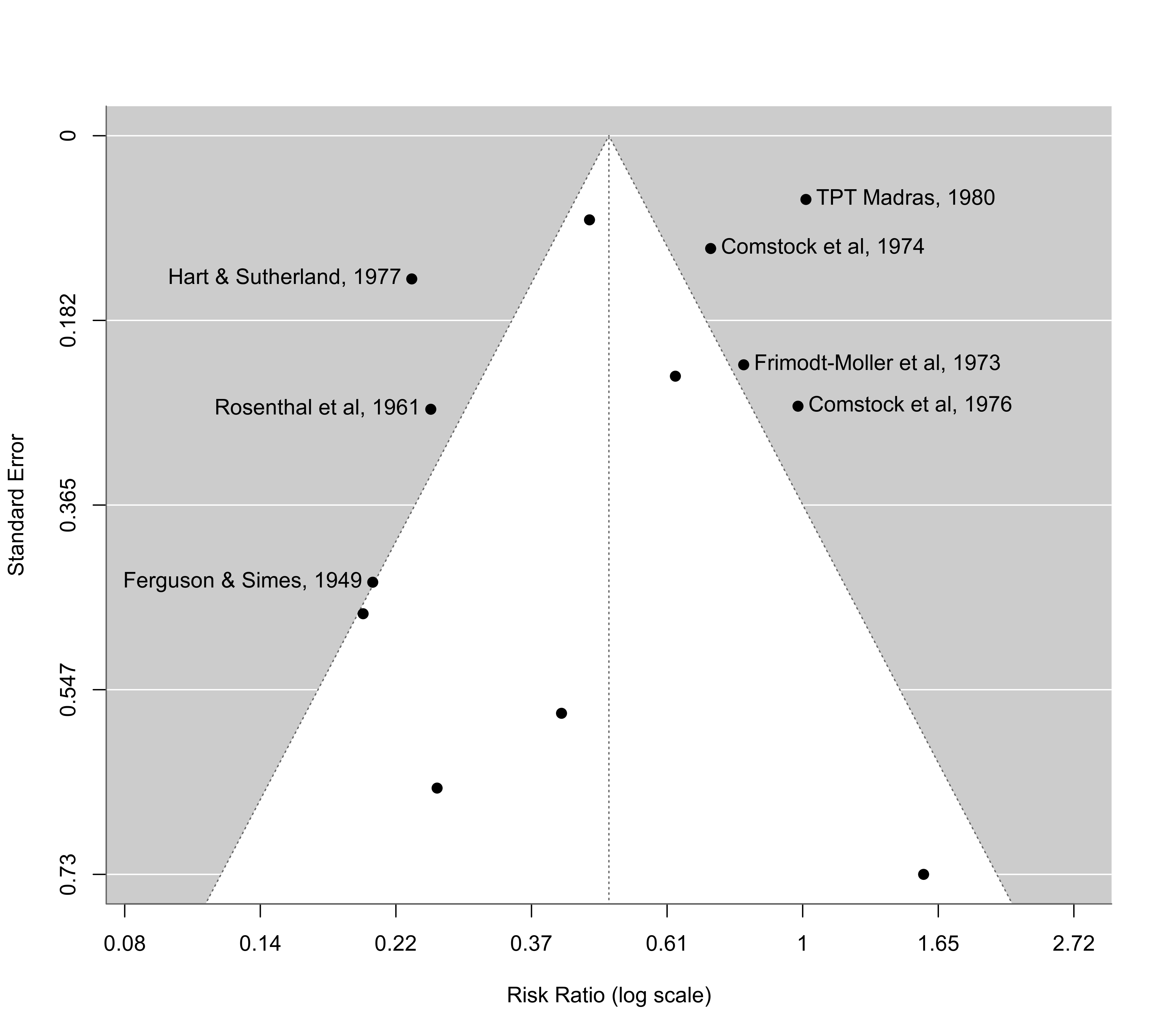
### copy BCG vaccine data into 'dat'
dat <- dat.bcg
### calculate log risk ratios and corresponding sampling variances
dat <- escalc(measure="RR", ai=tpos, bi=tneg, ci=cpos, di=cneg, data=dat)
### fit random-effects model
res <- rma(yi, vi, data=dat, slab=paste(author, year, sep=", "))
### draw a standard funnel plot
funnel(res)
 ### show risk ratio values on x-axis (log scale)
funnel(res, atransf=exp)
### label points outside of the pseudo confidence interval region
funnel(res, atransf=exp, label="out")
### show risk ratio values on x-axis (log scale)
funnel(res, atransf=exp)
### label points outside of the pseudo confidence interval region
funnel(res, atransf=exp, label="out")
 ### passing log risk ratios and sampling variances directly to the function
### note: same plot, except that the reference line is centered at zero
funnel(dat$yi, dat$vi)
### passing log risk ratios and sampling variances directly to the function
### note: same plot, except that the reference line is centered at zero
funnel(dat$yi, dat$vi)
 ### the with() function can be used to avoid having to retype dat$... over and over
with(dat, funnel(yi, vi))
### can accomplish the same thing by setting refline=0
funnel(res, refline=0)
### adjust the position of the x-axis labels, number of digits, and y-axis limits
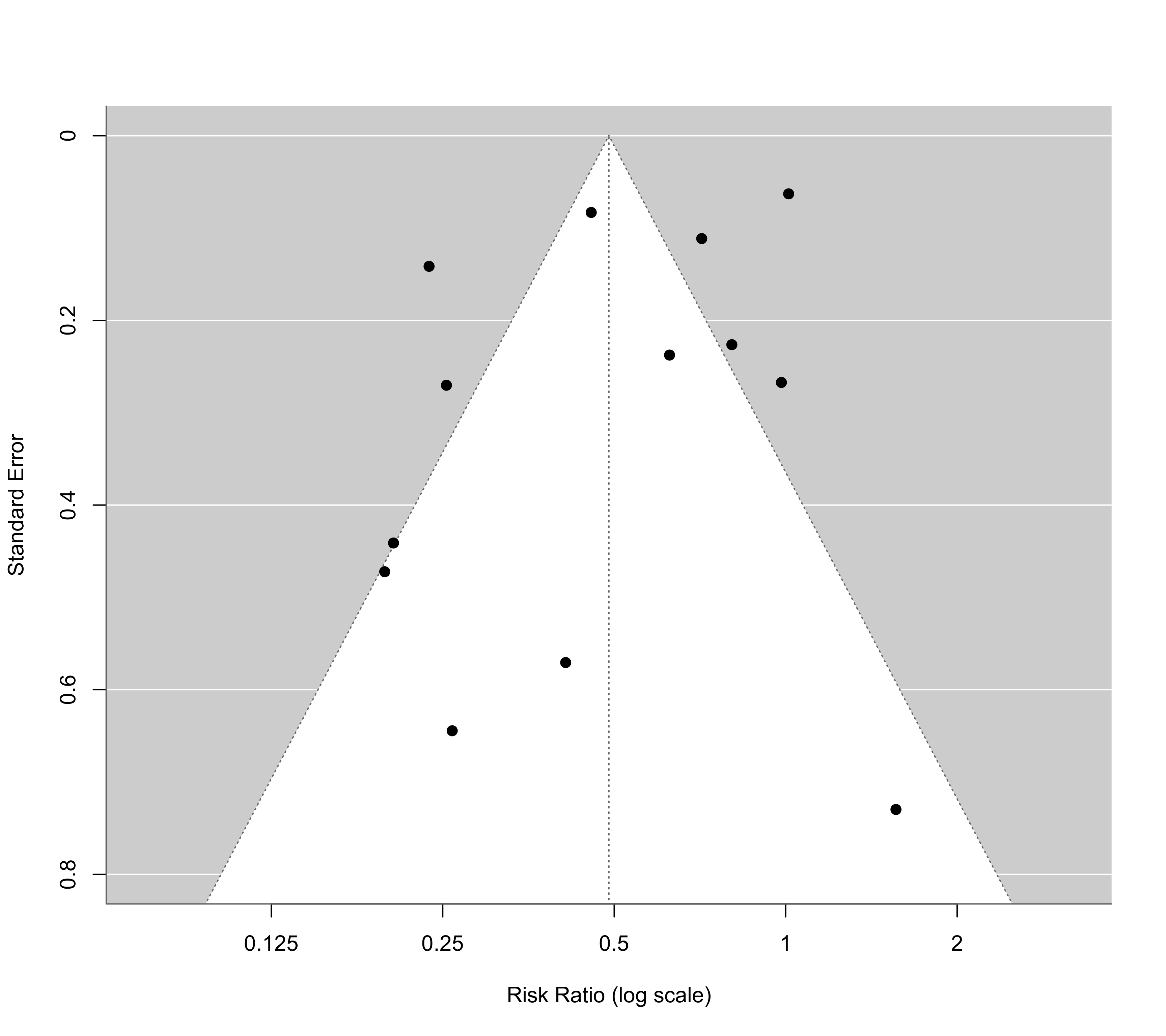
funnel(res, atransf=exp, at=log(c(0.125, 0.25, 0.5, 1, 2)), digits=3L, ylim=c(0,0.8))
### the with() function can be used to avoid having to retype dat$... over and over
with(dat, funnel(yi, vi))
### can accomplish the same thing by setting refline=0
funnel(res, refline=0)
### adjust the position of the x-axis labels, number of digits, and y-axis limits
funnel(res, atransf=exp, at=log(c(0.125, 0.25, 0.5, 1, 2)), digits=3L, ylim=c(0,0.8))
 ### contour-enhanced funnel plot centered at 0 (see Peters et al., 2008)
funnel(res, level=c(90, 95, 99), shade=c("white", "gray55", "gray75"), refline=0, legend=TRUE)
### contour-enhanced funnel plot centered at 0 (see Peters et al., 2008)
funnel(res, level=c(90, 95, 99), shade=c("white", "gray55", "gray75"), refline=0, legend=TRUE)
 ### default shades are chosen if the argument is not specified
funnel(res, level=c(90, 95, 99), refline=0, legend=TRUE)
### default shades are chosen if the argument is not specified
funnel(res, level=c(90, 95, 99), refline=0, legend=TRUE)
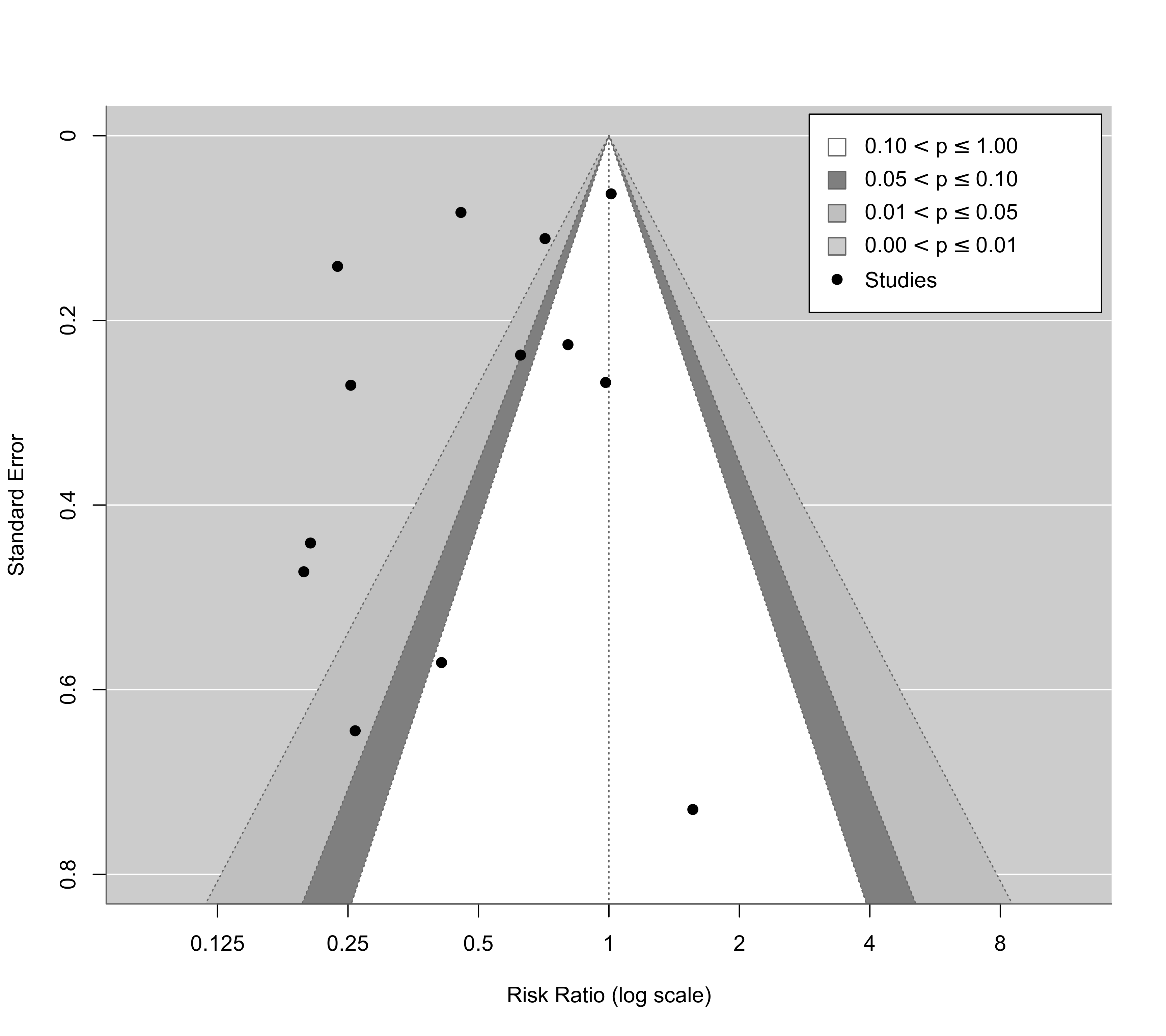
 ### same, but show risk ratio values on the x-axis and some further adjustments
funnel(res, level=c(90, 95, 99), digits=3L, ylim=c(0,0.8),
atransf=exp, at=log(c(0.125, 0.25, 0.5, 1, 2, 4, 8)), refline=0, legend=TRUE)
### same, but show risk ratio values on the x-axis and some further adjustments
funnel(res, level=c(90, 95, 99), digits=3L, ylim=c(0,0.8),
atransf=exp, at=log(c(0.125, 0.25, 0.5, 1, 2, 4, 8)), refline=0, legend=TRUE)
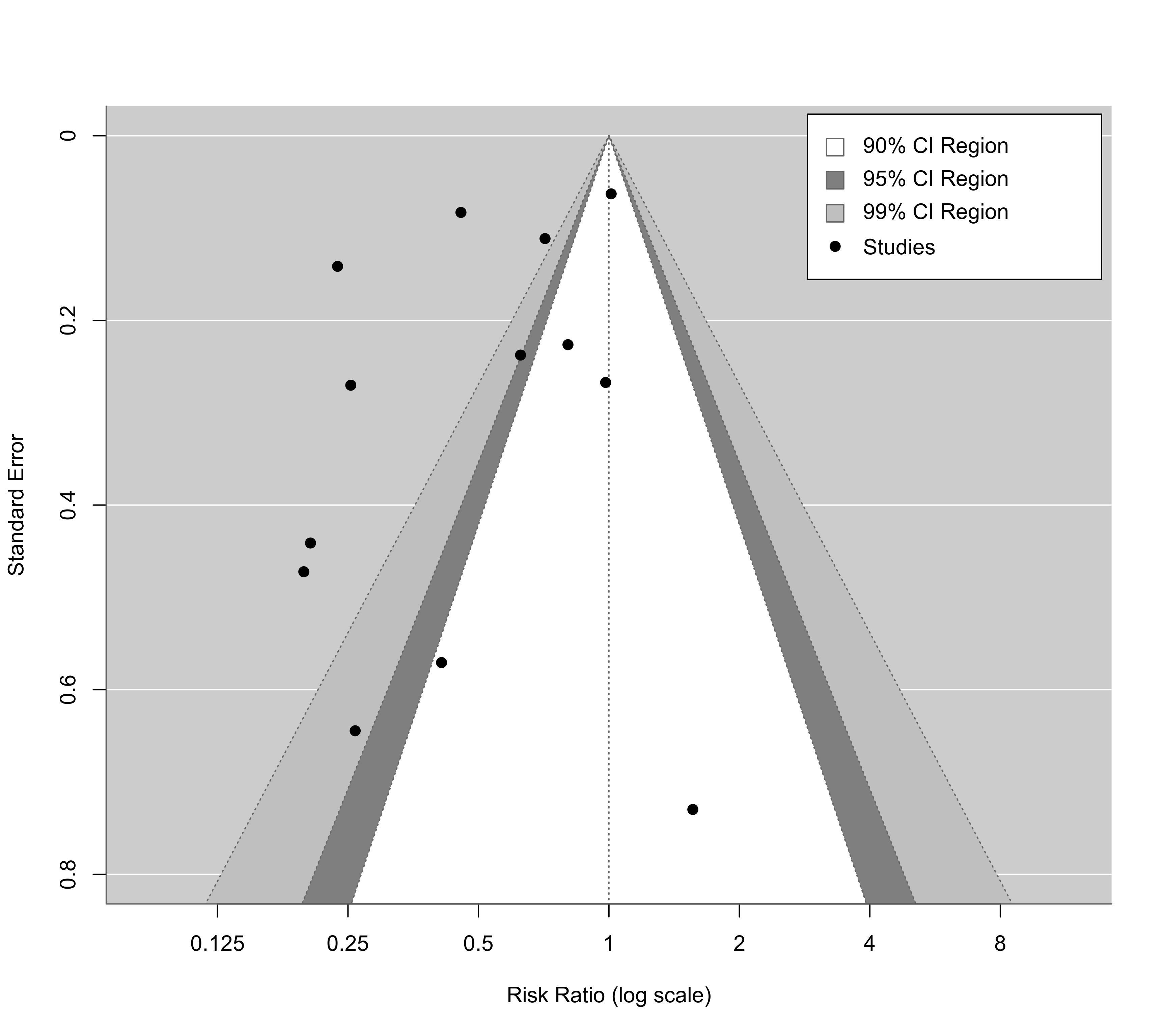
 ### same, but show confidence interval levels in the legend
funnel(res, level=c(90, 95, 99), digits=3L, ylim=c(0,0.8),
atransf=exp, at=log(c(0.125, 0.25, 0.5, 1, 2, 4, 8)), refline=0, legend=list(show="cis"))
### same, but show confidence interval levels in the legend
funnel(res, level=c(90, 95, 99), digits=3L, ylim=c(0,0.8),
atransf=exp, at=log(c(0.125, 0.25, 0.5, 1, 2, 4, 8)), refline=0, legend=list(show="cis"))
 ### illustrate the use of vectors for 'pch' and 'col'
res <- rma(yi, vi, data=dat, subset=2:10)
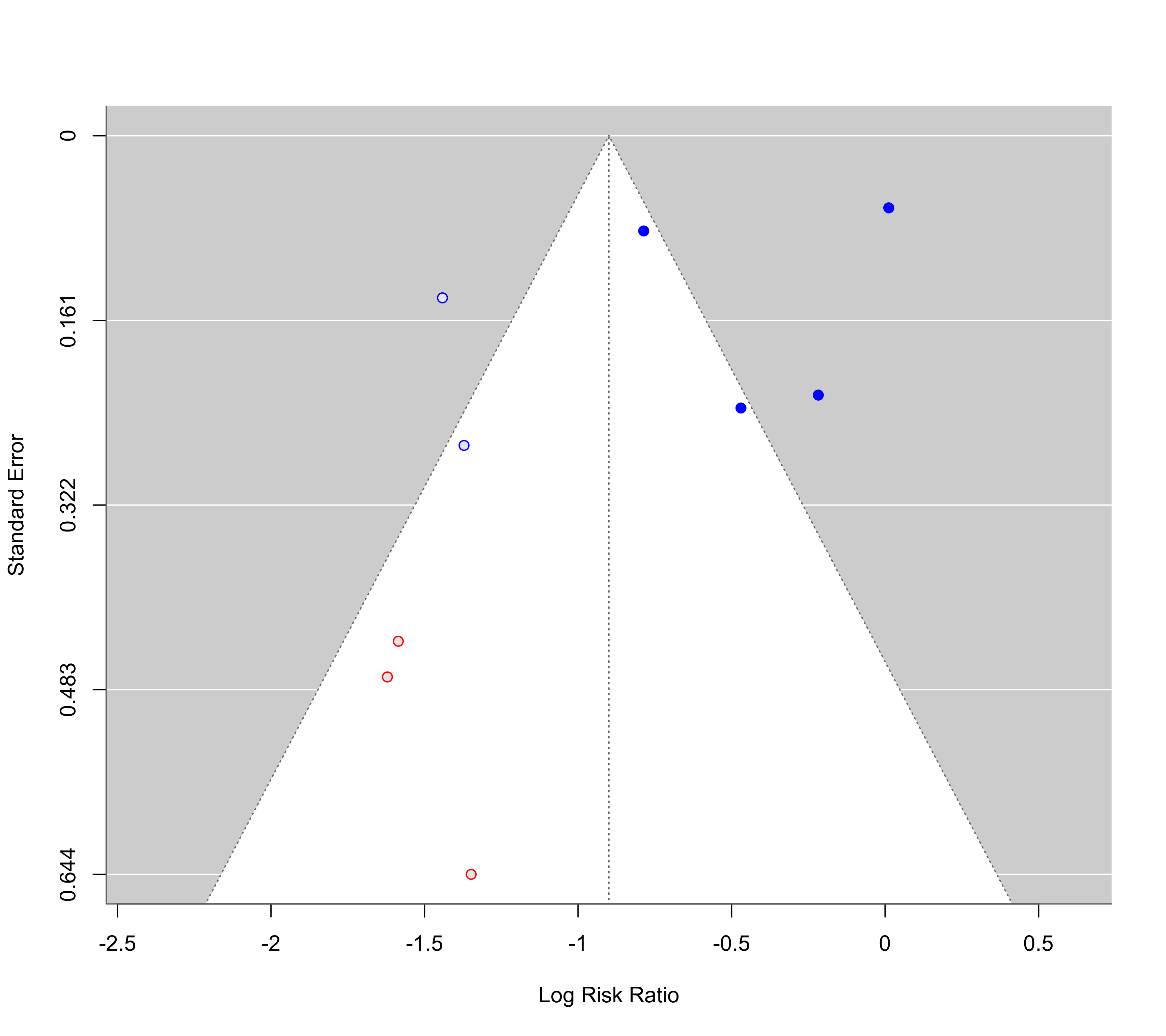
funnel(res, pch=ifelse(yi > -1, 19, 21), col=ifelse(sqrt(vi) > 0.3, "red", "blue"))
### illustrate the use of vectors for 'pch' and 'col'
res <- rma(yi, vi, data=dat, subset=2:10)
funnel(res, pch=ifelse(yi > -1, 19, 21), col=ifelse(sqrt(vi) > 0.3, "red", "blue"))
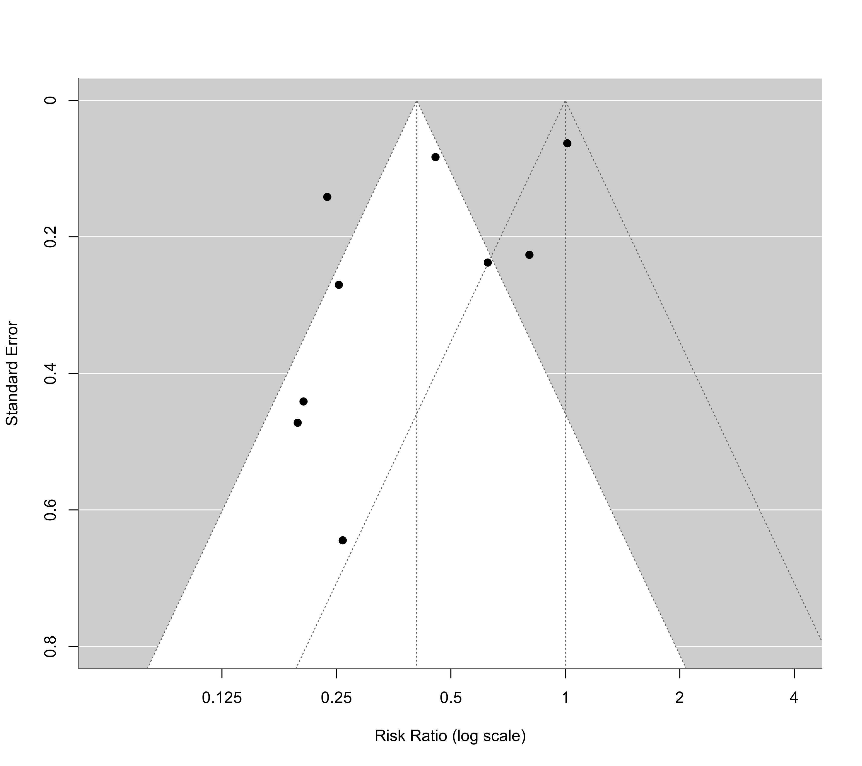
 ### can add a second funnel via (undocumented) argument refline2
funnel(res, atransf=exp, at=log(c(0.125, 0.25, 0.5, 1, 2, 4)), digits=3L, ylim=c(0,0.8), refline2=0)
### can add a second funnel via (undocumented) argument refline2
funnel(res, atransf=exp, at=log(c(0.125, 0.25, 0.5, 1, 2, 4)), digits=3L, ylim=c(0,0.8), refline2=0)
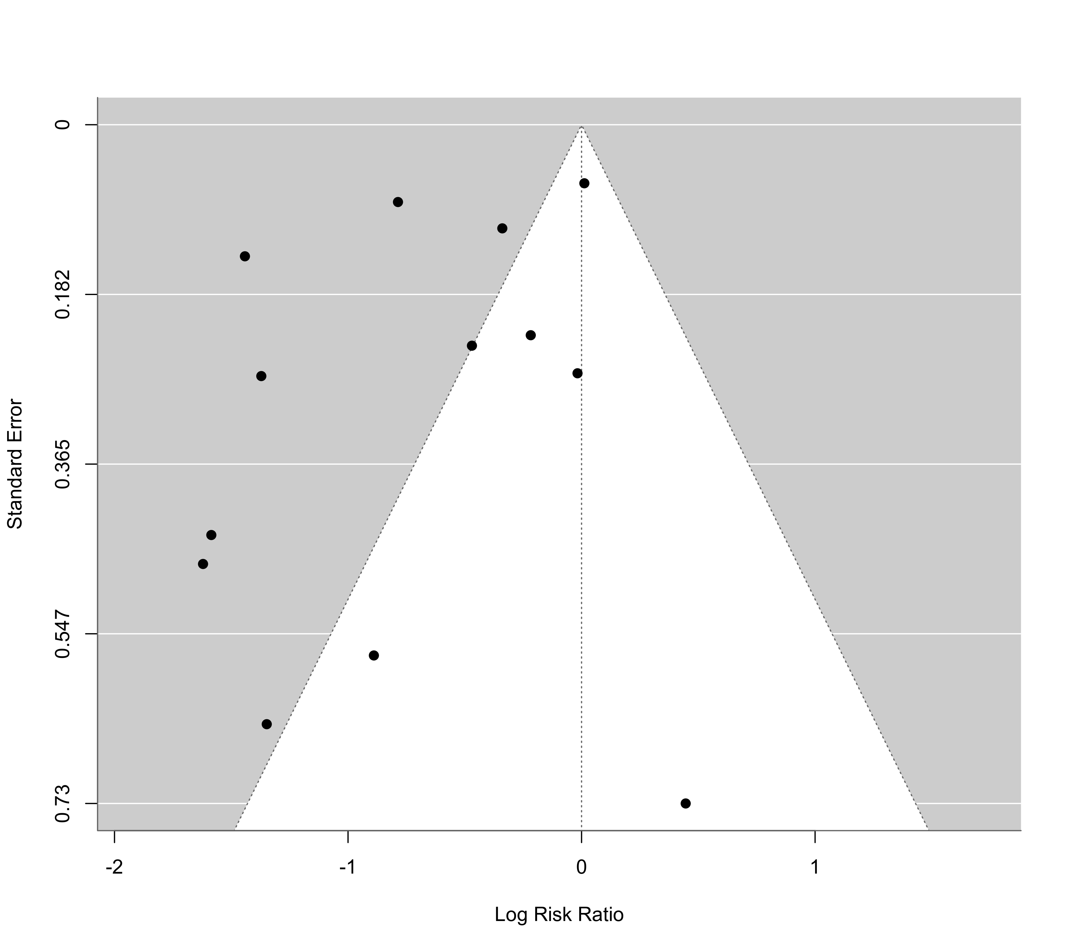
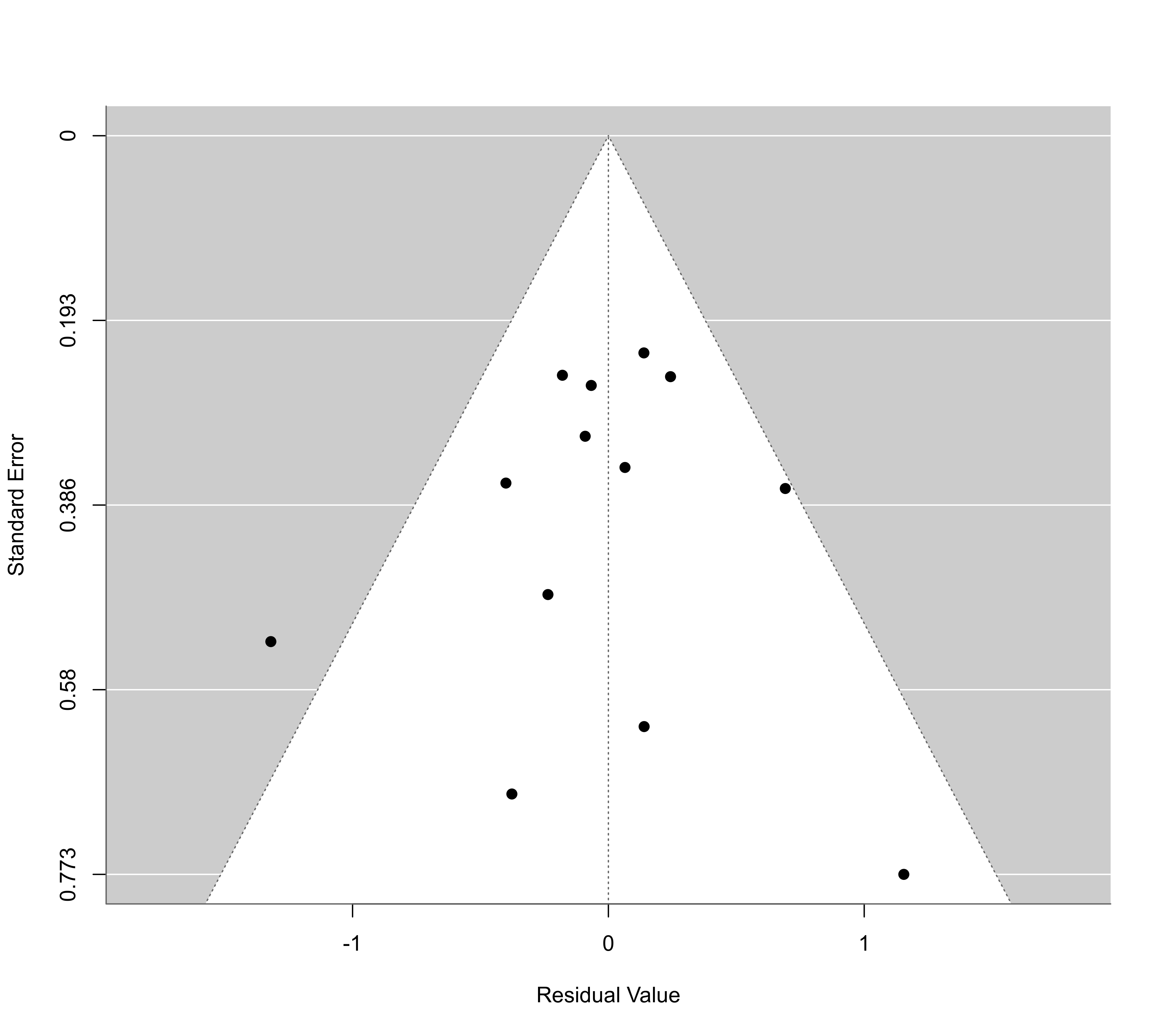
 ### mixed-effects model with absolute latitude in the model
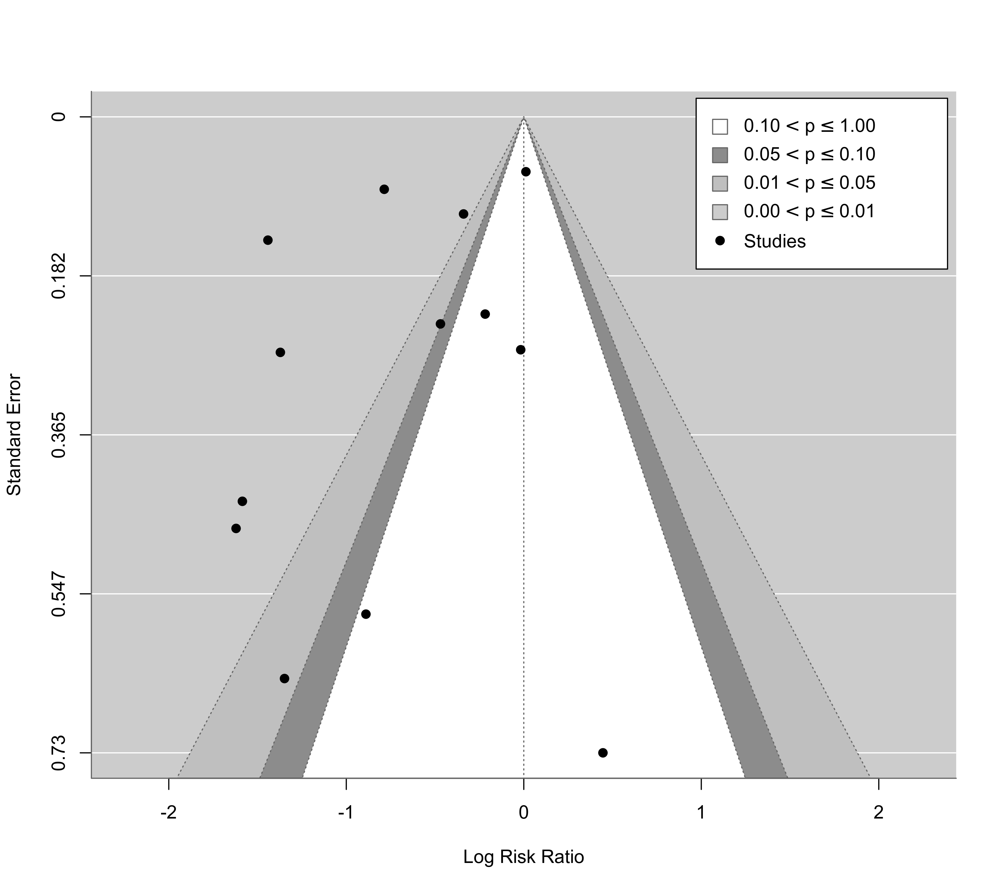
res <- rma(yi, vi, mods = ~ ablat, data=dat)
### funnel plot of the residuals
funnel(res)
### mixed-effects model with absolute latitude in the model
res <- rma(yi, vi, mods = ~ ablat, data=dat)
### funnel plot of the residuals
funnel(res)
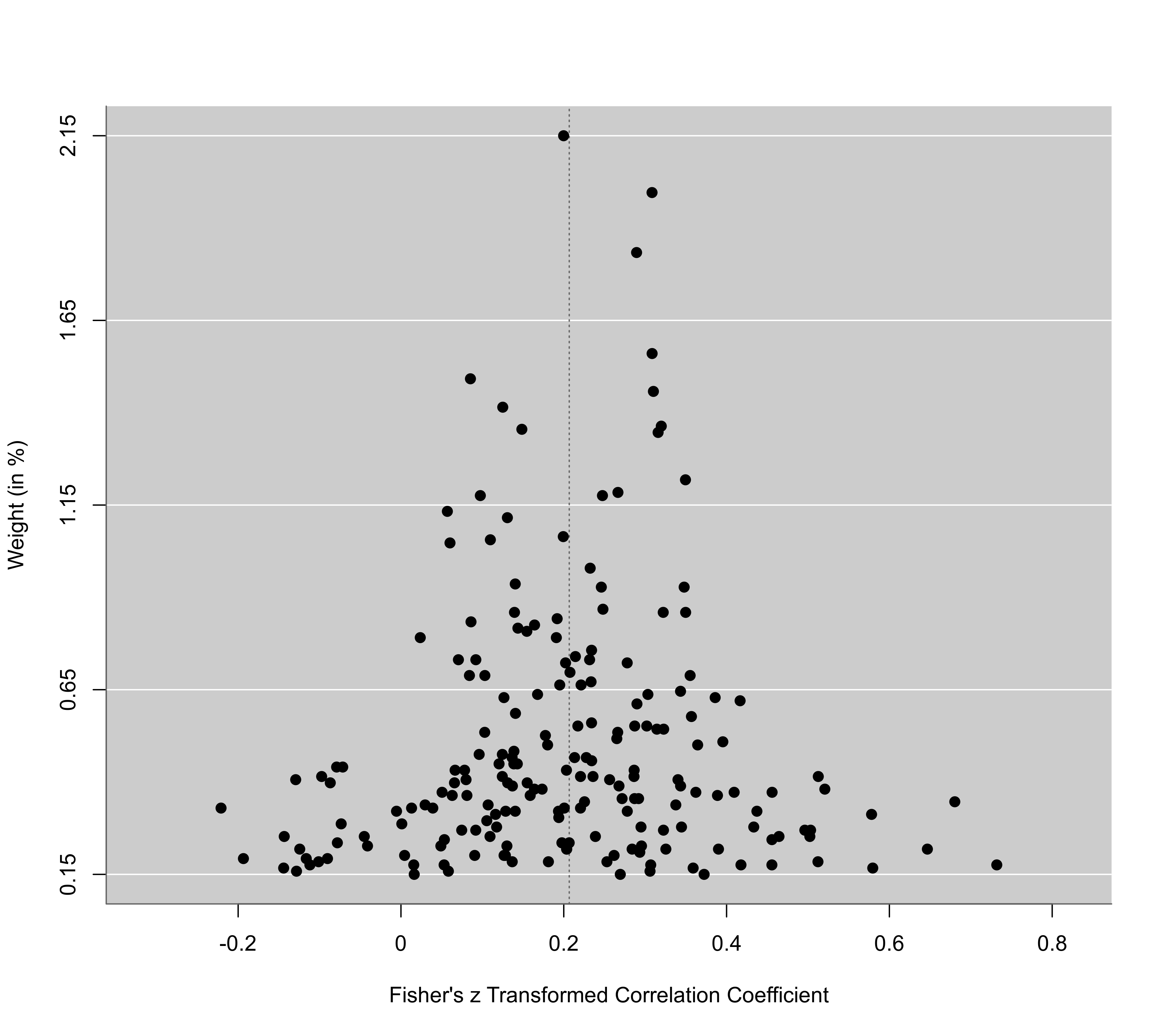
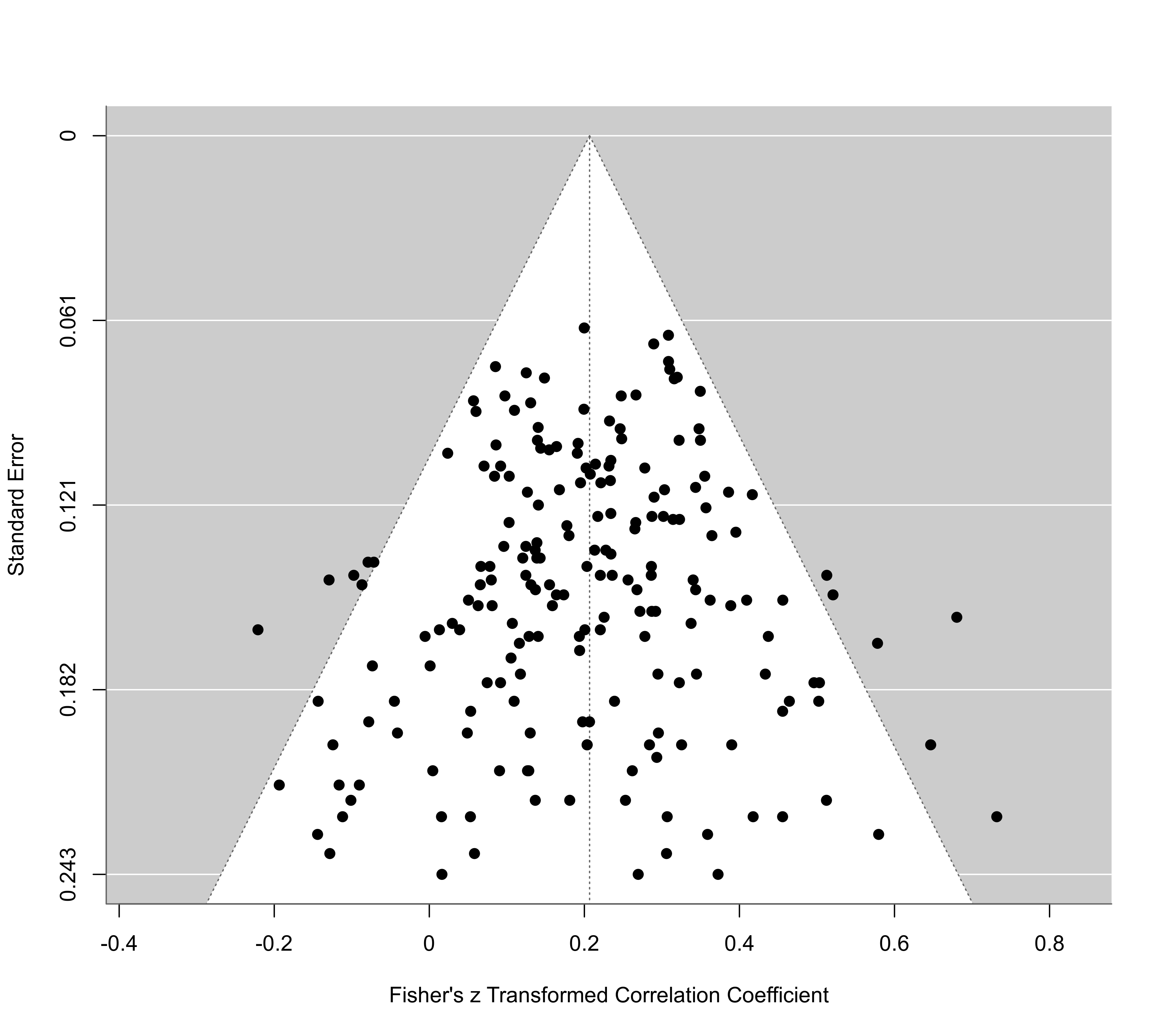
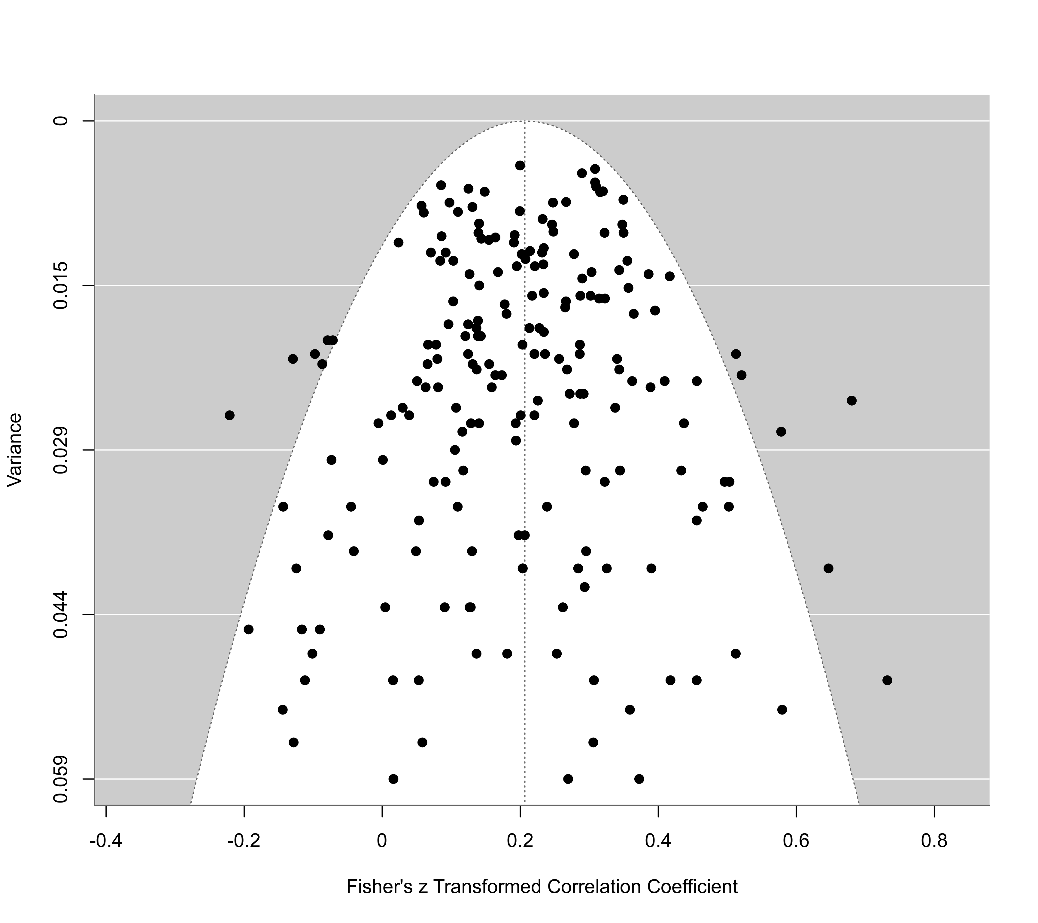
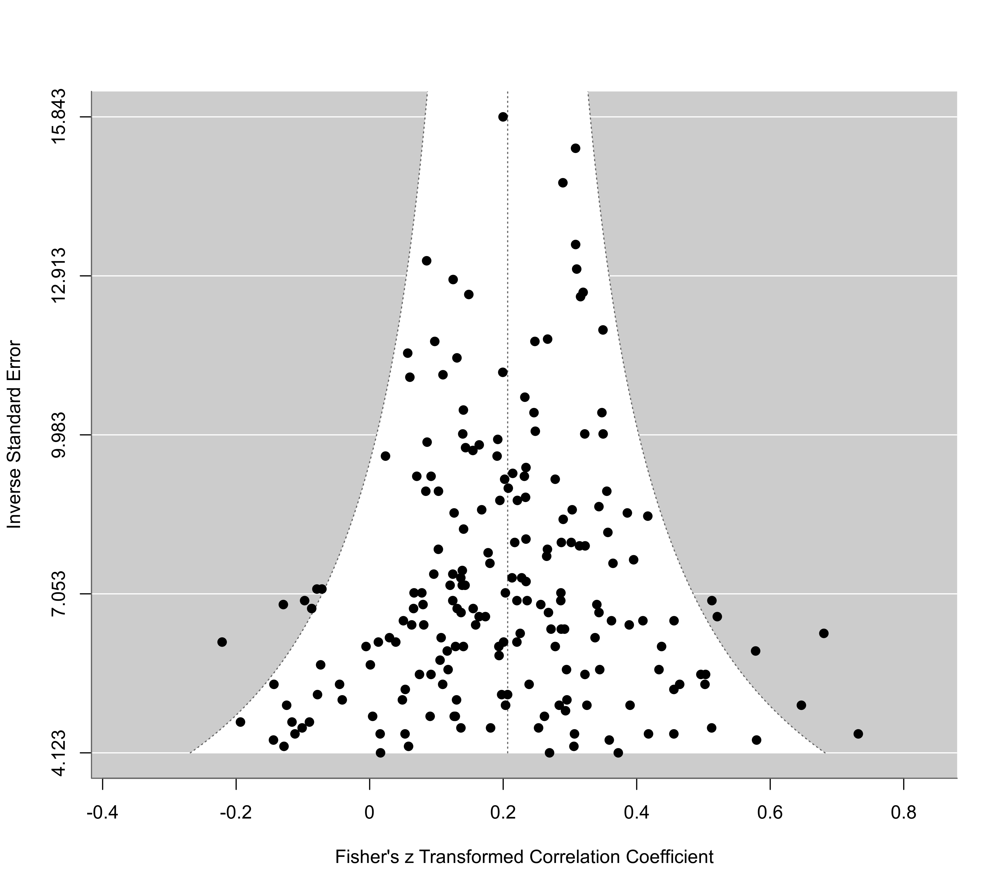
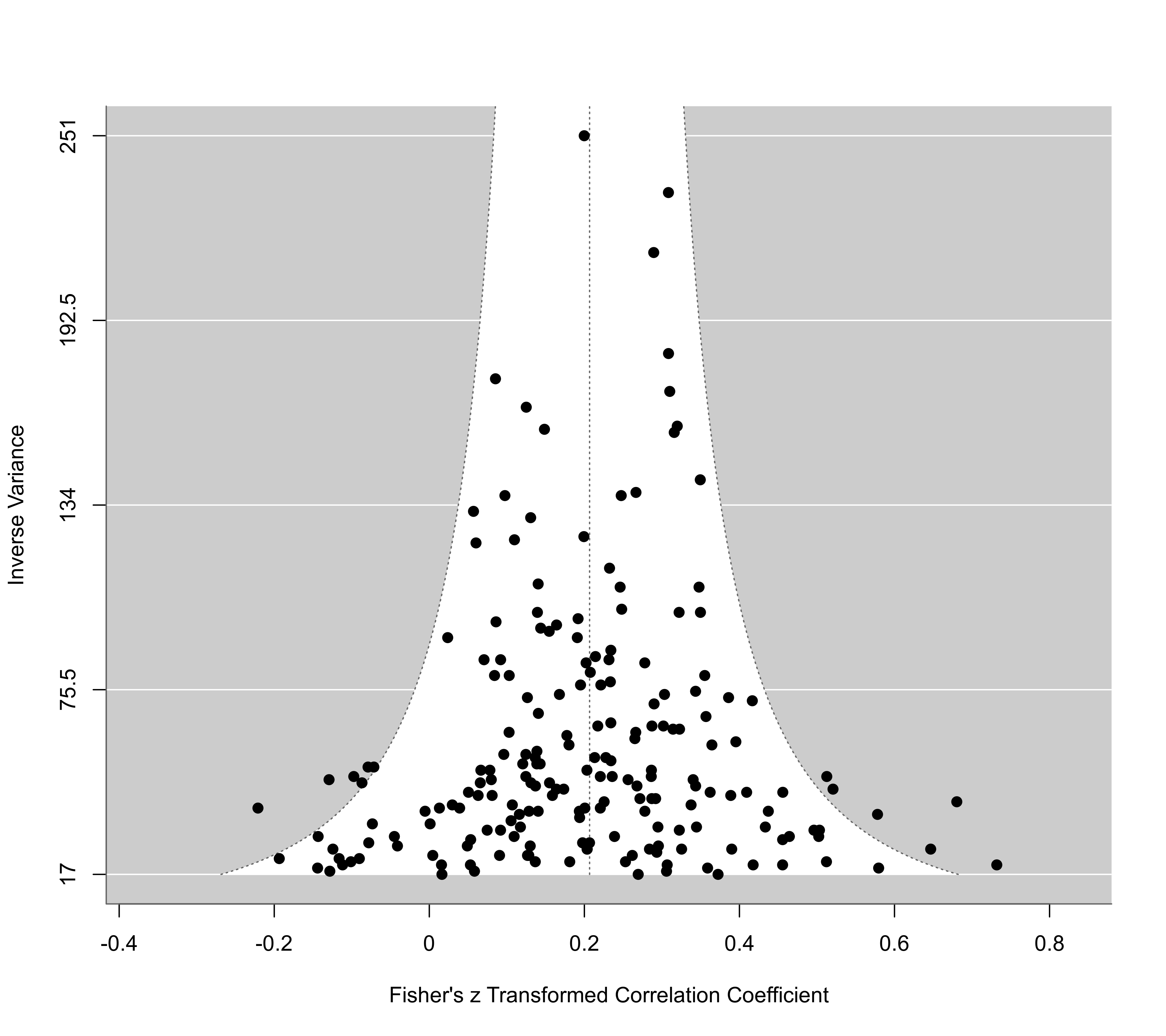
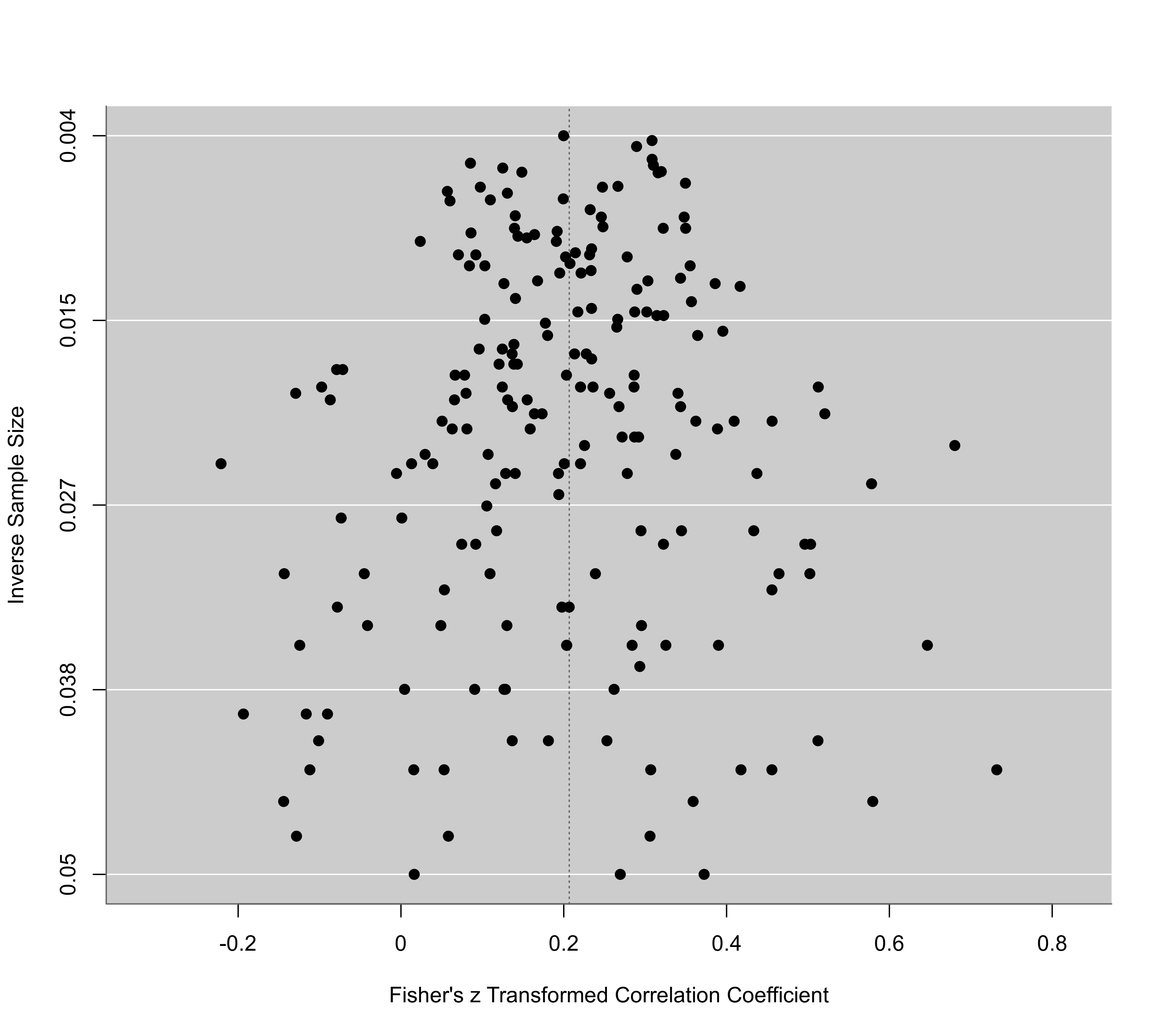
 ### simulate a large meta-analytic dataset (correlations with rho = 0.2)
### with no heterogeneity or publication bias; then try out different
### versions of the funnel plot
gencor <- function(rhoi, ni) {
x1 <- rnorm(ni, mean=0, sd=1)
x2 <- rnorm(ni, mean=0, sd=1)
x3 <- rhoi*x1 + sqrt(1-rhoi^2)*x2
cor(x1, x3)
}
set.seed(1234)
k <- 200 # number of studies to simulate
ni <- round(rchisq(k, df=2) * 20 + 20) # simulate sample sizes (skewed distribution)
ri <- mapply(gencor, rep(0.2,k), ni) # simulate correlations
res <- rma(measure="ZCOR", ri=ri, ni=ni, method="EE") # use r-to-z transformed correlations
funnel(res, yaxis="sei")
### simulate a large meta-analytic dataset (correlations with rho = 0.2)
### with no heterogeneity or publication bias; then try out different
### versions of the funnel plot
gencor <- function(rhoi, ni) {
x1 <- rnorm(ni, mean=0, sd=1)
x2 <- rnorm(ni, mean=0, sd=1)
x3 <- rhoi*x1 + sqrt(1-rhoi^2)*x2
cor(x1, x3)
}
set.seed(1234)
k <- 200 # number of studies to simulate
ni <- round(rchisq(k, df=2) * 20 + 20) # simulate sample sizes (skewed distribution)
ri <- mapply(gencor, rep(0.2,k), ni) # simulate correlations
res <- rma(measure="ZCOR", ri=ri, ni=ni, method="EE") # use r-to-z transformed correlations
funnel(res, yaxis="sei")
 funnel(res, yaxis="vi")
 funnel(res, yaxis="seinv")
 funnel(res, yaxis="vinv")
 funnel(res, yaxis="ni")
 funnel(res, yaxis="ninv")
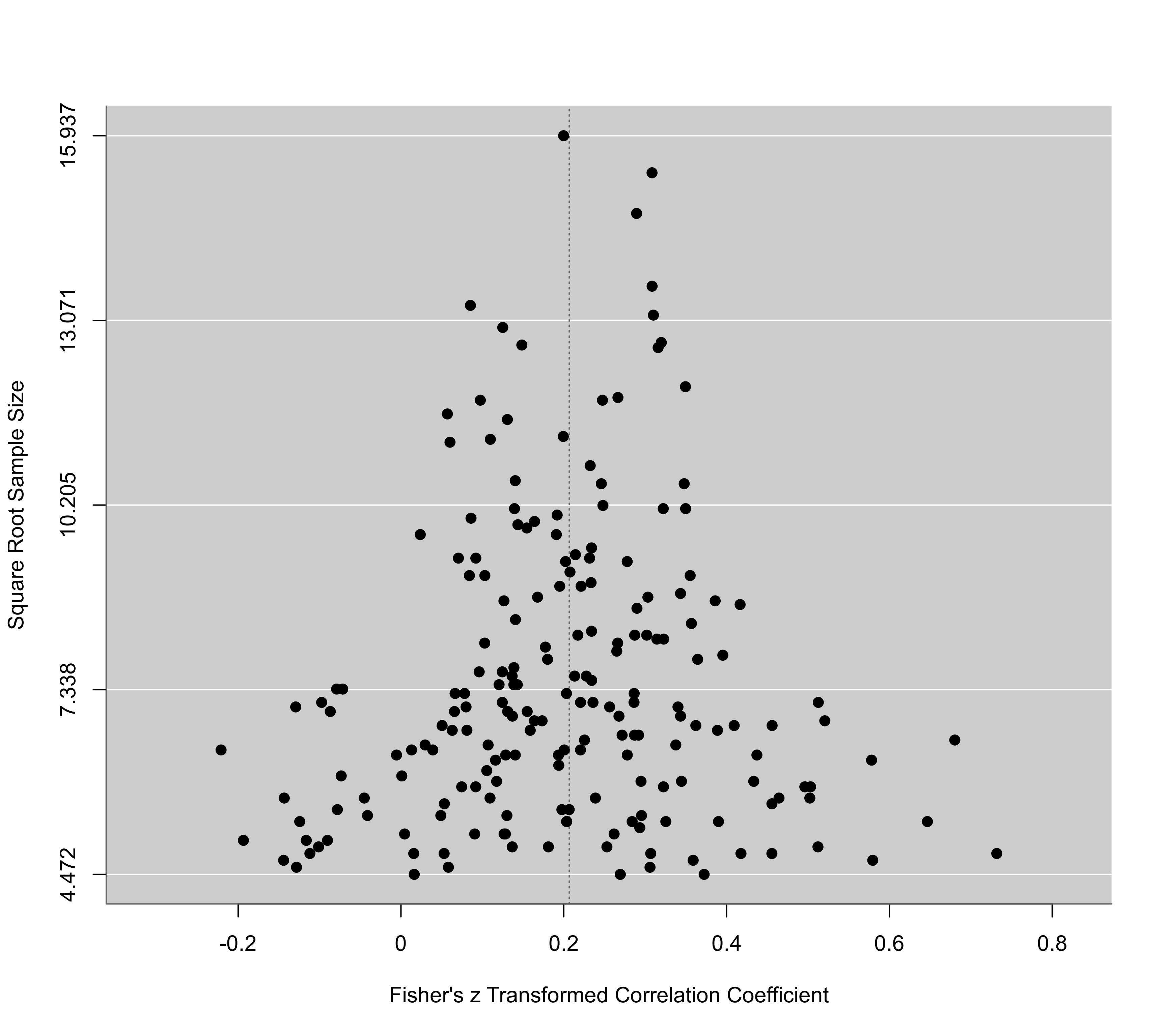
 funnel(res, yaxis="sqrtni")
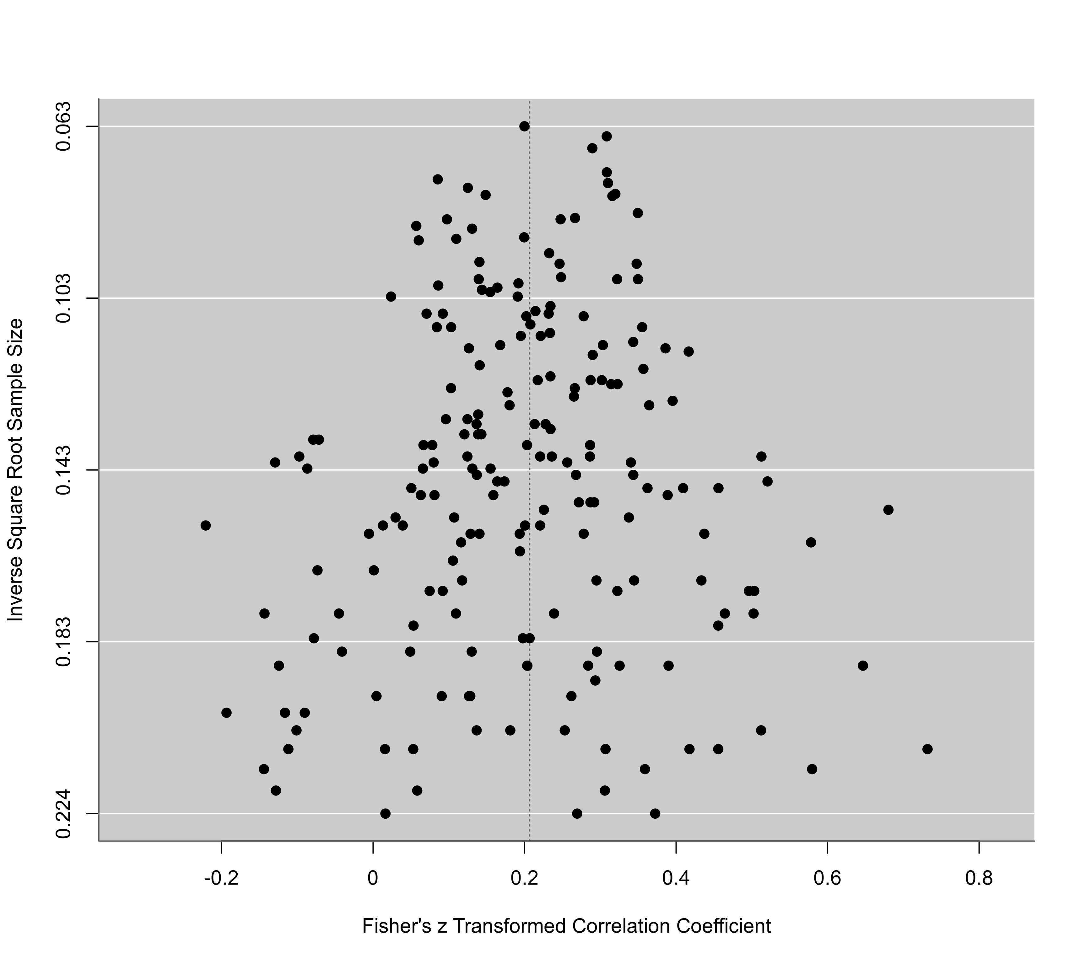
 funnel(res, yaxis="sqrtninv")
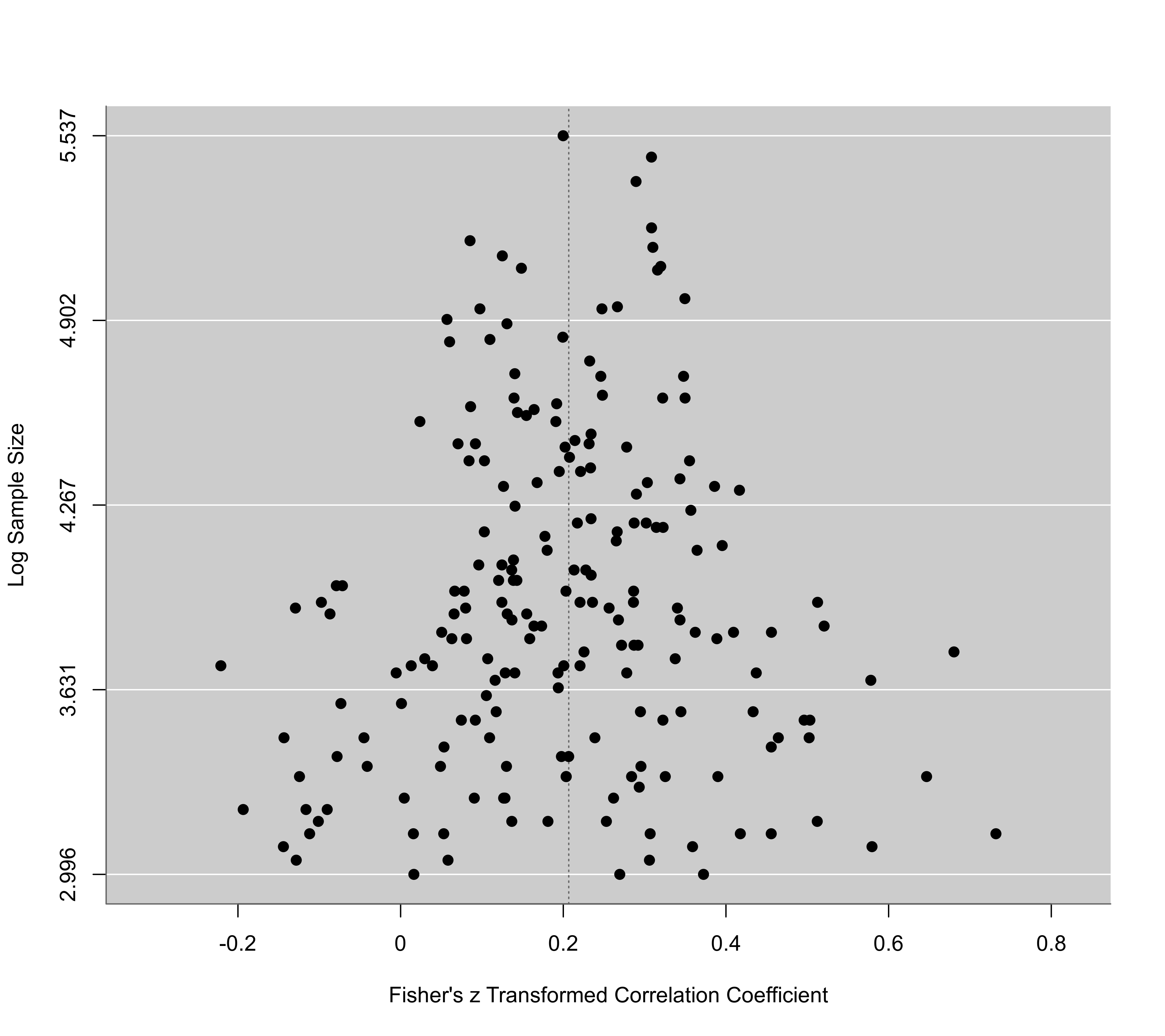
 funnel(res, yaxis="lni")
 funnel(res, yaxis="wi")