Meta-Analysis based on the Method by Henmi and Copas (2010)

Function to obtain an estimate of the average true outcome and corresponding confidence interval under a random-effects model using the method described by Henmi and Copas (2010).

hc(object, ...)

# S3 method for rma.uni
hc(object, digits, transf, targs, control, ...)

Arguments

object: an object of class "rma.uni".
digits: optional integer to specify the number of decimal places to which the printed results should be rounded. If unspecified, the default is to take the value from the object.
transf: optional argument to specify a function to transform the estimate and the corresponding interval bounds (e.g., transf=exp; see also transf). If unspecified, no transformation is used.
targs: optional arguments needed by the function specified under transf.
control: list of control values for the iterative algorithm. If unspecified, default values are used. See ‘Note’.
...: other arguments.

Details

The model specified via object must be a model without moderators (i.e., either an equal- or a random-effects model).

When using the usual method for fitting a random-effects model (i.e., weighted estimation with inverse-variance weights), the weights assigned to smaller and larger studies become more uniform as the amount of heterogeneity increases. As a consequence, the estimated average outcome could become increasingly biased under certain forms of publication bias (where smaller studies on one side of the funnel plot are missing). The method by Henmi and Copas (2010) counteracts this problem by providing an estimate of the average true outcome that is based on inverse-variance weights as used under an equal-effects model, which are not affected by the amount of heterogeneity. The amount of heterogeneity is still estimated (with the DerSimonian-Laird estimator) and incorporated into the standard error of the estimated average outcome and the corresponding confidence interval.

Currently, there is only a method for handling objects of class "rma.uni" with the hc function. It therefore provides a method for conducting a sensitivity analysis after the model has been fitted with the rma.uni function.

Value

An object of class "hc.rma.uni". The object is a list containing the following components:

beta: estimated average true outcome.
se: corresponding standard error.
ci.lb: lower bound of the confidence intervals for the average true outcome.
ci.ub: upper bound of the confidence intervals for the average true outcome.
...: some additional elements/values.

The results are formatted and printed with the print function.

Note

The method makes use of the uniroot function. By default, the desired accuracy is set equal to .Machine$double.eps^0.25 and the maximum number of iterations to 1000. The desired accuracy (tol) and the maximum number of iterations (maxiter) can be adjusted with the control argument (i.e., control=list(tol=value, maxiter=value)).

Author

Original code by Henmi and Copas (2010). Corrected for typos by Michael Dewey (lists@dewey.myzen.co.uk). Incorporated into the package with some small adjustments for consistency with the other functions in the package by Wolfgang Viechtbauer (wvb@metafor-project.org).

References

Henmi, M., & Copas, J. B. (2010). Confidence intervals for random effects meta-analysis and robustness to publication bias. Statistics in Medicine, 29(29), 2969–2983. https://doi.org/10.1002/sim.4029

Viechtbauer, W. (2010). Conducting meta-analyses in R with the metafor package. Journal of Statistical Software, 36(3), 1–48. https://doi.org/10.18637/jss.v036.i03

Examples

### calculate log odds ratios and corresponding sampling variances
dat <- escalc(measure="OR", ai=ai, n1i=n1i, ci=ci, n2i=n2i, data=dat.lee2004)
dat
#> 
#>    id        study year ai n1i ci n2i      yi     vi 
#> 1   1      Agarwal 2000 18 100 20 100 -0.1301 0.1303 
#> 2   2      Agarwal 2002  5  50 18  50 -1.6219 0.3090 
#> 3   3     Alkaissi 1999  9  20  7  20  0.4184 0.4218 
#> 4   4     Alkaissi 2002 32 135 31 139  0.0792 0.0825 
#> 5   5        Allen 1994  9  23 10  23 -0.1795 0.3595 
#> 6   6 Andrzejowski 1996 11  18 12  18 -0.2412 0.4838 
#> 7   7       Duggal 1998 69 122 80 122 -0.3805 0.0697 
#> 8   8       Dundee 1986  3  25 12  25 -1.9124 0.5390 
#> 9   9 Ferrera-Love 1996  1  30  1  30  0.0000 2.0690 
#> 10 10       Gieron 1993 11  30 19  30 -1.0931 0.2871 
#> 11 11       Harmon 1999  7  44 16  39 -1.3021 0.2759 
#> 12 12       Harmon 2000  4  47  6  47 -0.4531 0.4643 
#> 13 13           Ho 1996  1  30 13  30 -3.0990 1.1702 
#> 14 14         Rusy 2002 24  40 71  80 -1.6600 0.2294 
#> 15 15         Wang 2002 16  50 53  88 -1.1687 0.1394 
#> 16 16       Zarate 2001 28 110 25 111  0.1610 0.0995 
#> 

### meta-analysis based on log odds ratios
res <- rma(yi, vi, data=dat)
res
#> 
#> Random-Effects Model (k = 16; tau^2 estimator: REML)
#> 
#> tau^2 (estimated amount of total heterogeneity): 0.3526 (SE = 0.2254)
#> tau (square root of estimated tau^2 value):      0.5938
#> I^2 (total heterogeneity / total variability):   62.35%
#> H^2 (total variability / sampling variability):  2.66
#> 
#> Test for Heterogeneity:
#> Q(df = 15) = 38.4231, p-val = 0.0008
#> 
#> Model Results:
#> 
#> estimate      se     zval    pval    ci.lb    ci.ub      
#>  -0.6820  0.2013  -3.3877  0.0007  -1.0766  -0.2874  *** 
#> 
#> ---
#> Signif. codes:  0 ‘***’ 0.001 ‘**’ 0.01 ‘*’ 0.05 ‘.’ 0.1 ‘ ’ 1
#> 

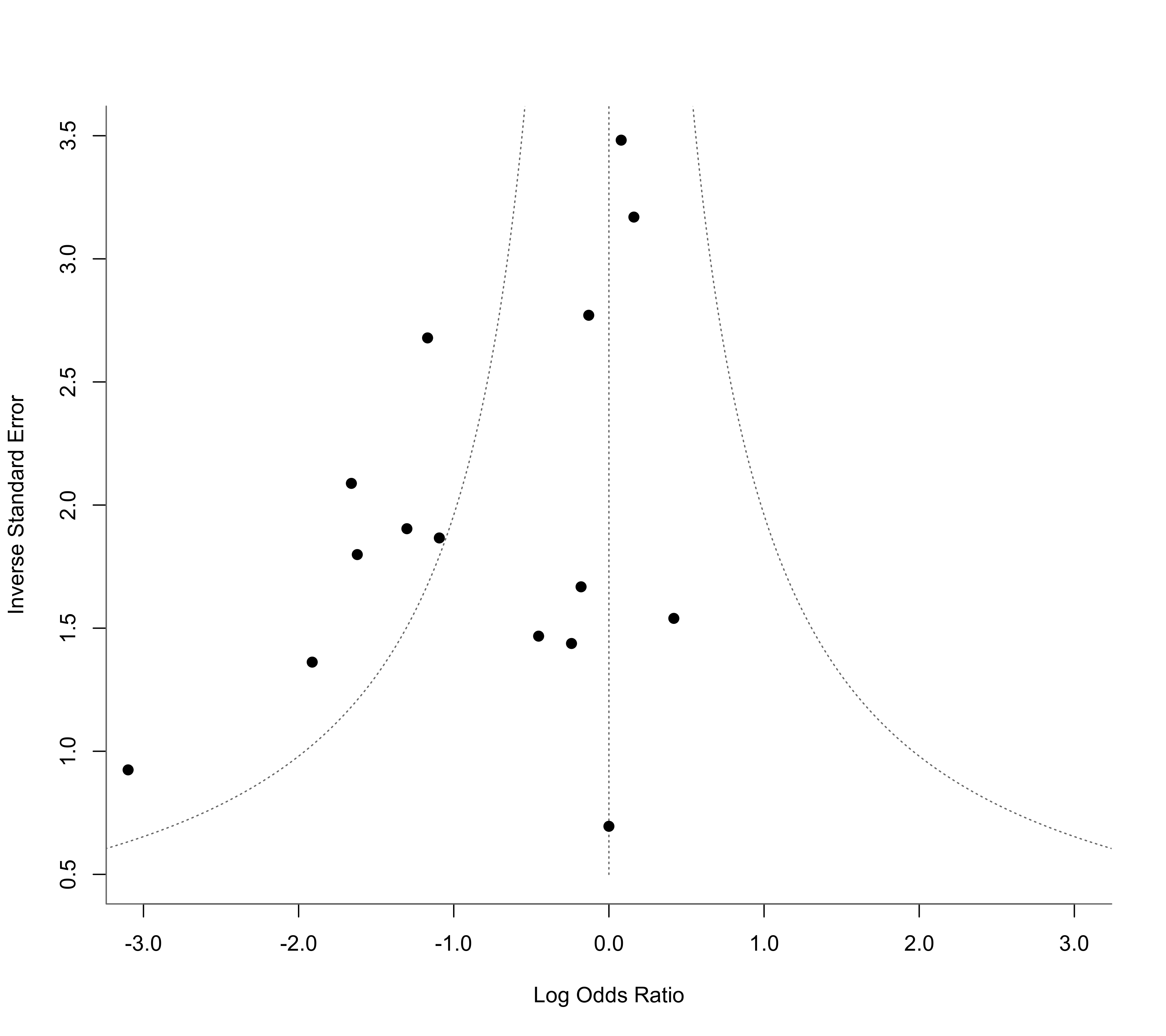
### funnel plot as in Henmi and Copas (2010)
funnel(res, yaxis="seinv", refline=0, xlim=c(-3,3), ylim=c(.5,3.5), steps=7, digits=1, back="white")


### use method by Henmi and Copas (2010) as a sensitivity analysis
hc(res)
#> 
#>     method   tau2 estimate     se   ci.lb   ci.ub 
#> rma   REML 0.3526  -0.6820 0.2013 -1.0766 -0.2874 
#> hc      DL 0.3325  -0.5145 0.2178 -0.9994 -0.0295 
#> 

### back-transform results to odds ratio scale
hc(res, transf=exp)
#> 
#>     method   tau2 estimate  ci.lb  ci.ub 
#> rma   REML 0.3526   0.5056 0.3408 0.7502 
#> hc      DL 0.3325   0.5978 0.3681 0.9709 
#>