Studies on the Accuracy of Venous Ultrasonography for the Diagnosis of Deep Venous Thrombosis
dat.kearon1998.RdResults from diagnostic accuracy studies examining the accuracy of venous ultrasonography for the diagnosis of deep venous thrombosis.
dat.kearon1998Format
The data frame contains the following columns:
| id | numeric | study id |
| author | character | study author(s) |
| year | numeric | publication year |
| patients | character | patient group (either symptomatic or asymptomatic patients) |
| tp | numeric | number of true positives |
| np | numeric | number of positive patients (cases) |
| tn | numeric | number of true negatives |
| nn | numeric | number of negative patients (non-cases) |
Details
The studies included in the dataset examined the accuracy of venous ultrasonography for the diagnossis of a first deep venous thrombosis in symptomatic and asymptomatic patients. Cases and non-cases were determined based on contrast venography. Venous ultrasonography was then used to make a diagnosis, leading to a given number of true positives and negatives.
A subset of this dataset (using only the studies with asymptomatic patients) was used by Deeks et al. (2005) to illustrate methods for detecting publication bias (or small-study effects) in meta-analyses of diagnostic accuracy studies.
Source
Kearon, C., Julian, J. A., Math, M., Newman, T. E., & Ginsberg, J. S. (1998). Noninvasive diagnosis of deep venous thrombosis. Annals of Internal Medicine, 128(8), 663–677. https://doi.org/10.7326/0003-4819-128-8-199804150-00011
References
Deeks, J. J., Macaskill, P., & Irwig, L. (2005). The performance of tests of publication bias and other sample size effects in systematic reviews of diagnostic test accuracy was assessed. Journal of Clinical Epidemiology, 58(9), 882–893. https://doi.org/10.1016/j.jclinepi.2005.01.016
Concepts
medicine, odds ratios, diagnostic accuracy studies, multivariate models, publication bias
Examples
### copy data into 'dat' and examine data
dat <- dat.kearon1998
head(dat)
#> id study year patients tp np tn nn
#> 1 1 Elias et al. 1987 symptomatic 325 333 483 505
#> 2 2 Appleman et al. 1987 symptomatic NA NA 47 49
#> 3 3 Vogel et al. 1987 symptomatic 20 25 29 29
#> 4 4 Cronan et al. 1987 symptomatic 25 28 23 23
#> 5 5 O'Leary et al. 1988 symptomatic 22 25 24 25
#> 6 6 Lensing et al. 1989 symptomatic 70 77 142 143
### load metafor package
library(metafor)
### calculate diagnostic log odds ratios and corresponding sampling variances
dat <- escalc(measure="OR", ai=tp, n1i=np, ci=nn-tn, n2i=nn, data=dat, add=1/2, to="all")
head(dat)
#>
#> id study year patients tp np tn nn yi vi
#> 1 1 Elias et al. 1987 symptomatic 325 333 483 505 6.7128 0.1672
#> 2 2 Appleman et al. 1987 symptomatic NA NA 47 49 NA NA
#> 3 3 Vogel et al. 1987 symptomatic 20 25 29 29 5.3932 2.2645
#> 4 4 Cronan et al. 1987 symptomatic 25 28 23 23 5.8361 2.3675
#> 5 5 O'Leary et al. 1988 symptomatic 22 25 24 25 4.6540 1.0376
#> 6 6 Lensing et al. 1989 symptomatic 70 77 142 143 6.7946 0.8212
#>
### fit random-effects model for the symptomatic patients
res <- rma(yi, vi, data=dat, subset=patients=="symptomatic")
#> Warning: 2 studies with NAs omitted from model fitting.
res
#>
#> Random-Effects Model (k = 16; tau^2 estimator: REML)
#>
#> tau^2 (estimated amount of total heterogeneity): 1.2663 (SE = 0.7846)
#> tau (square root of estimated tau^2 value): 1.1253
#> I^2 (total heterogeneity / total variability): 66.20%
#> H^2 (total variability / sampling variability): 2.96
#>
#> Test for Heterogeneity:
#> Q(df = 15) = 48.8101, p-val < .0001
#>
#> Model Results:
#>
#> estimate se zval pval ci.lb ci.ub
#> 5.1733 0.3747 13.8057 <.0001 4.4388 5.9077 ***
#>
#> ---
#> Signif. codes: 0 ‘***’ 0.001 ‘**’ 0.01 ‘*’ 0.05 ‘.’ 0.1 ‘ ’ 1
#>
### fit random-effects model for the asymptomatic patients
res <- rma(yi, vi, data=dat, subset=patients=="asymptomatic")
#> Warning: 2 studies with NAs omitted from model fitting.
res
#>
#> Random-Effects Model (k = 14; tau^2 estimator: REML)
#>
#> tau^2 (estimated amount of total heterogeneity): 0.4534 (SE = 0.3776)
#> tau (square root of estimated tau^2 value): 0.6734
#> I^2 (total heterogeneity / total variability): 48.58%
#> H^2 (total variability / sampling variability): 1.94
#>
#> Test for Heterogeneity:
#> Q(df = 13) = 28.3304, p-val = 0.0081
#>
#> Model Results:
#>
#> estimate se zval pval ci.lb ci.ub
#> 3.0039 0.2682 11.2017 <.0001 2.4783 3.5295 ***
#>
#> ---
#> Signif. codes: 0 ‘***’ 0.001 ‘**’ 0.01 ‘*’ 0.05 ‘.’ 0.1 ‘ ’ 1
#>
### estimated average diagnostic odds ratio (with 95% CI)
predict(res, transf=exp, digits=2)
#>
#> pred ci.lb ci.ub pi.lb pi.ub
#> 20.16 11.92 34.11 4.87 83.47
#>
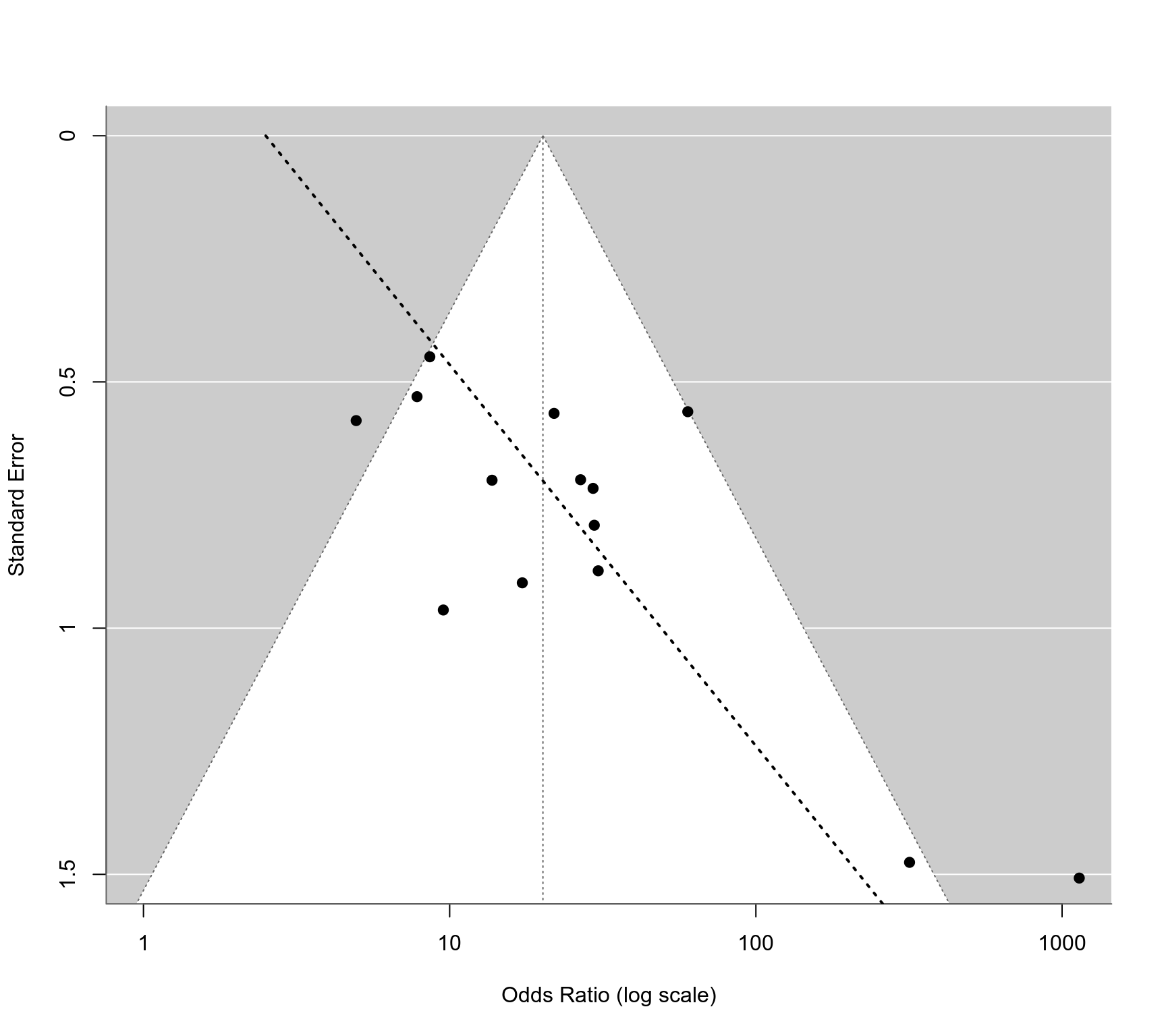
### regression test for funnel plot asymmetry using SE as predictor
reg <- regtest(res, model="lm")
reg
#>
#> Regression Test for Funnel Plot Asymmetry
#>
#> Model: weighted regression with multiplicative dispersion
#> Predictor: standard error
#>
#> Test for Funnel Plot Asymmetry: t = 2.7886, df = 12, p = 0.0164
#> Limit Estimate (as sei -> 0): b = 0.9192 (CI: -0.6698, 2.5082)
#>
### corresponding funnel plot
funnel(res, atransf=exp, xlim=c(0,7), at=log(c(1,10,100,1000)), ylim=c(0,1.5), steps=4)
ys <- seq(0, 2, length=100)
lines(coef(reg$fit)[1] + coef(reg$fit)[2]*ys, ys, lwd=2, lty=3)
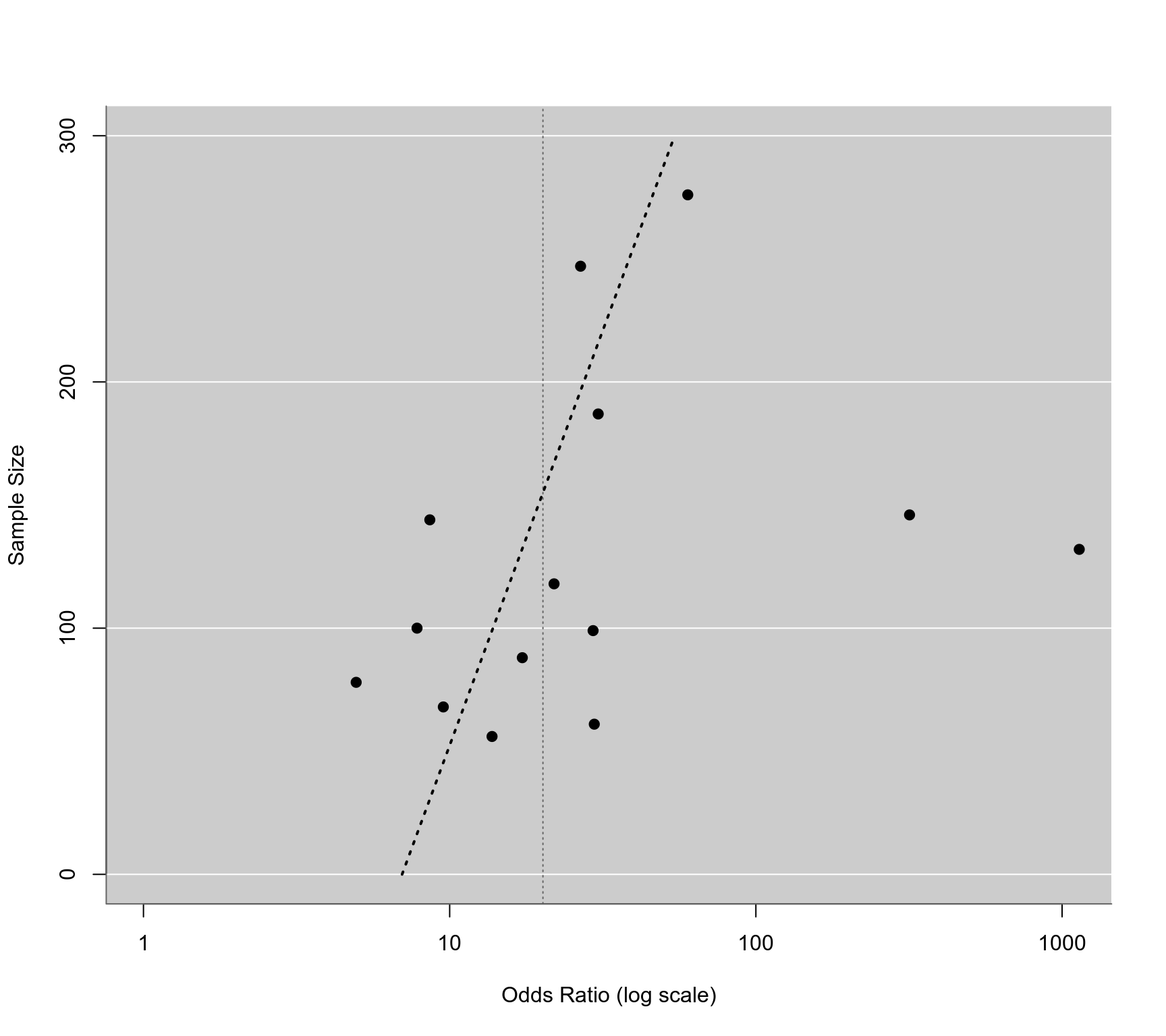
 ### regression test for funnel plot asymmetry using total sample size as predictor
reg <- regtest(res, model="lm", predictor="ni")
reg
#>
#> Regression Test for Funnel Plot Asymmetry
#>
#> Model: weighted regression with multiplicative dispersion
#> Predictor: sample size
#>
#> Test for Funnel Plot Asymmetry: t = 1.8919, df = 12, p = 0.0829
#>
### corresponding funnel plot
funnel(res, yaxis="ni", atransf=exp, xlim=c(0,7), at=log(c(1,10,100,1000)), ylim=c(0,300), steps=4)
ys <- seq(0, 300, length=100)
lines(coef(reg$fit)[1] + coef(reg$fit)[2]*ys, ys, lwd=2, lty=3)
### regression test for funnel plot asymmetry using total sample size as predictor
reg <- regtest(res, model="lm", predictor="ni")
reg
#>
#> Regression Test for Funnel Plot Asymmetry
#>
#> Model: weighted regression with multiplicative dispersion
#> Predictor: sample size
#>
#> Test for Funnel Plot Asymmetry: t = 1.8919, df = 12, p = 0.0829
#>
### corresponding funnel plot
funnel(res, yaxis="ni", atransf=exp, xlim=c(0,7), at=log(c(1,10,100,1000)), ylim=c(0,300), steps=4)
ys <- seq(0, 300, length=100)
lines(coef(reg$fit)[1] + coef(reg$fit)[2]*ys, ys, lwd=2, lty=3)
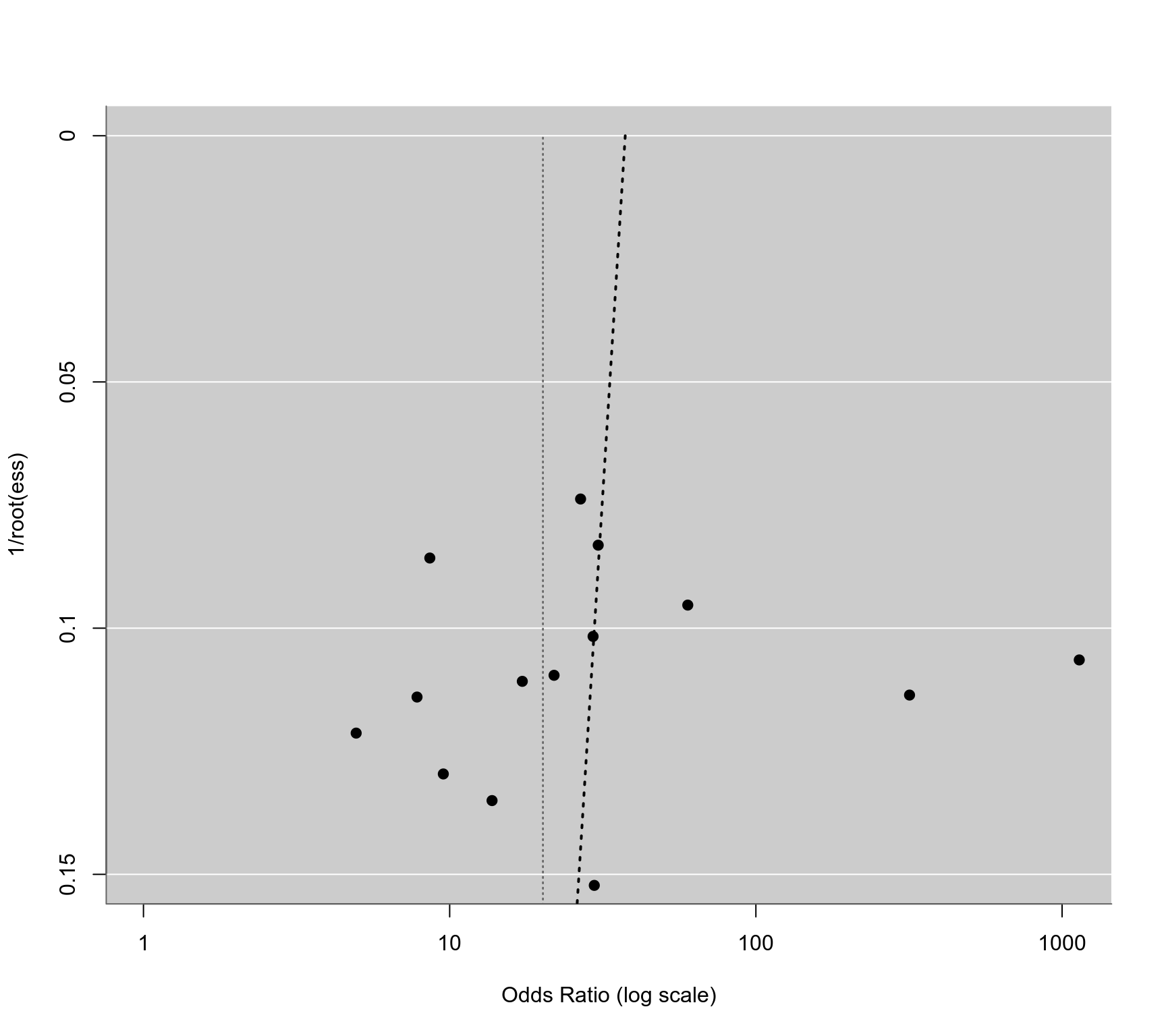
 ### regression test for funnel plot asymmetry using 1/sqrt(ESS) as predictor (Deeks et al., 2005)
dat$invessi <- 1/(4*dat$np) + 1/(4*dat$nn)
tmp <- rma(yi, invessi, data=dat, subset=patients=="asymptomatic")
#> Warning: 2 studies with NAs omitted from model fitting.
reg <- regtest(tmp, model="lm")
reg
#>
#> Regression Test for Funnel Plot Asymmetry
#>
#> Model: weighted regression with multiplicative dispersion
#> Predictor: standard error
#>
#> Test for Funnel Plot Asymmetry: t = -0.1182, df = 12, p = 0.9079
#> Limit Estimate (as sei -> 0): b = 3.6227 (CI: -0.8066, 8.0520)
#>
### corresponding funnel plot
funnel(tmp, atransf=exp, xlim=c(0,7), at=log(c(1,10,100,1000)), ylim=c(0,0.15), steps=4,
refline=coef(res), level=0, ylab="1/root(ess)")
ys <- seq(0, 0.2, length=100)
lines(coef(reg$fit)[1] + coef(reg$fit)[2]*ys, ys, lwd=2, lty=3)
### regression test for funnel plot asymmetry using 1/sqrt(ESS) as predictor (Deeks et al., 2005)
dat$invessi <- 1/(4*dat$np) + 1/(4*dat$nn)
tmp <- rma(yi, invessi, data=dat, subset=patients=="asymptomatic")
#> Warning: 2 studies with NAs omitted from model fitting.
reg <- regtest(tmp, model="lm")
reg
#>
#> Regression Test for Funnel Plot Asymmetry
#>
#> Model: weighted regression with multiplicative dispersion
#> Predictor: standard error
#>
#> Test for Funnel Plot Asymmetry: t = -0.1182, df = 12, p = 0.9079
#> Limit Estimate (as sei -> 0): b = 3.6227 (CI: -0.8066, 8.0520)
#>
### corresponding funnel plot
funnel(tmp, atransf=exp, xlim=c(0,7), at=log(c(1,10,100,1000)), ylim=c(0,0.15), steps=4,
refline=coef(res), level=0, ylab="1/root(ess)")
ys <- seq(0, 0.2, length=100)
lines(coef(reg$fit)[1] + coef(reg$fit)[2]*ys, ys, lwd=2, lty=3)
 ### convert data to long format
dat <- to.long(measure="OR", ai=tp, n1i=np, ci=tn, n2i=nn,
data=dat.kearon1998, subset=patients=="asymptomatic", append=FALSE)
#> Warning: 2 tables with NAs omitted.
dat$group <- factor(dat$group, levels=c(1,2), labels=c("sensitivity", "specificity"))
dat
#> study group out1 out2
#> 1 19 sensitivity 10 15
#> 2 19 specificity 47 6
#> 3 20 sensitivity 15 9
#> 4 20 specificity 29 3
#> 5 21 sensitivity 10 4
#> 6 21 specificity 44 3
#> 7 22 sensitivity 13 10
#> 8 22 specificity 123 0
#> 9 23 sensitivity 10 22
#> 10 23 specificity 55 1
#> 11 24 sensitivity 16 45
#> 12 24 specificity 184 2
#> 13 25 sensitivity 12 37
#> 14 25 specificity 137 1
#> 15 26 sensitivity 13 13
#> 16 26 specificity 66 8
#> 17 28 sensitivity 24 18
#> 18 28 specificity 55 2
#> 19 29 sensitivity 17 10
#> 20 29 specificity 85 6
#> 21 30 sensitivity 5 17
#> 22 30 specificity 45 1
#> 23 31 sensitivity 18 13
#> 24 31 specificity 240 5
#> 25 32 sensitivity 24 4
#> 26 32 specificity 104 0
#> 27 33 sensitivity 26 29
#> 28 33 specificity 81 8
### calculate logit-transformed sensitivities
dat <- escalc(measure="PLO", xi=out1, mi=out2, data=dat, add=1/2, to="all",
include=group=="sensitivity")
dat
#>
#> study group out1 out2 yi vi
#> 1 19 sensitivity 10 15 -0.3895 0.1598
#> 2 19 specificity 47 6 NA NA
#> 3 20 sensitivity 15 9 0.4895 0.1698
#> 4 20 specificity 29 3 NA NA
#> 5 21 sensitivity 10 4 0.8473 0.3175
#> 6 21 specificity 44 3 NA NA
#> 7 22 sensitivity 13 10 0.2513 0.1693
#> 8 22 specificity 123 0 NA NA
#> 9 23 sensitivity 10 22 -0.7621 0.1397
#> 10 23 specificity 55 1 NA NA
#> 11 24 sensitivity 16 45 -1.0144 0.0826
#> 12 24 specificity 184 2 NA NA
#> 13 25 sensitivity 12 37 -1.0986 0.1067
#> 14 25 specificity 137 1 NA NA
#> 15 26 sensitivity 13 13 0.0000 0.1481
#> 16 26 specificity 66 8 NA NA
#> 17 28 sensitivity 24 18 0.2809 0.0949
#> 18 28 specificity 55 2 NA NA
#> 19 29 sensitivity 17 10 0.5108 0.1524
#> 20 29 specificity 85 6 NA NA
#> 21 30 sensitivity 5 17 -1.1575 0.2390
#> 22 30 specificity 45 1 NA NA
#> 23 31 sensitivity 18 13 0.3151 0.1281
#> 24 31 specificity 240 5 NA NA
#> 25 32 sensitivity 24 4 1.6946 0.2630
#> 26 32 specificity 104 0 NA NA
#> 27 33 sensitivity 26 29 -0.1072 0.0716
#> 28 33 specificity 81 8 NA NA
#>
### calculate logit-transformed specificities
dat <- escalc(measure="PLO", xi=out1, mi=out2, data=dat, add=1/2, to="all",
include=group=="specificity")
dat
#>
#> study group out1 out2 yi vi
#> 1 19 sensitivity 10 15 -0.3895 0.1598
#> 2 19 specificity 47 6 1.9889 0.1749
#> 3 20 sensitivity 15 9 0.4895 0.1698
#> 4 20 specificity 29 3 2.1316 0.3196
#> 5 21 sensitivity 10 4 0.8473 0.3175
#> 6 21 specificity 44 3 2.5427 0.3082
#> 7 22 sensitivity 13 10 0.2513 0.1693
#> 8 22 specificity 123 0 5.5094 2.0081
#> 9 23 sensitivity 10 22 -0.7621 0.1397
#> 10 23 specificity 55 1 3.6109 0.6847
#> 11 24 sensitivity 16 45 -1.0144 0.0826
#> 12 24 specificity 184 2 4.3014 0.4054
#> 13 25 sensitivity 12 37 -1.0986 0.1067
#> 14 25 specificity 137 1 4.5182 0.6739
#> 15 26 sensitivity 13 13 0.0000 0.1481
#> 16 26 specificity 66 8 2.0571 0.1327
#> 17 28 sensitivity 24 18 0.2809 0.0949
#> 18 28 specificity 55 2 3.1001 0.4180
#> 19 29 sensitivity 17 10 0.5108 0.1524
#> 20 29 specificity 85 6 2.5767 0.1655
#> 21 30 sensitivity 5 17 -1.1575 0.2390
#> 22 30 specificity 45 1 3.4122 0.6886
#> 23 31 sensitivity 18 13 0.3151 0.1281
#> 24 31 specificity 240 5 3.7780 0.1860
#> 25 32 sensitivity 24 4 1.6946 0.2630
#> 26 32 specificity 104 0 5.3423 2.0096
#> 27 33 sensitivity 26 29 -0.1072 0.0716
#> 28 33 specificity 81 8 2.2605 0.1299
#>
### bivariate random-effects model for logit sensitivity and specificity
res <- rma.mv(yi, vi, mods = ~ 0 + group, random = ~ group | study, struct="UN", data=dat)
res
#>
#> Multivariate Meta-Analysis Model (k = 28; method: REML)
#>
#> Variance Components:
#>
#> outer factor: study (nlvls = 14)
#> inner factor: group (nlvls = 2)
#>
#> estim sqrt k.lvl fixed level
#> tau^2.1 0.4231 0.6505 14 no sensitivity
#> tau^2.2 0.5408 0.7354 14 no specificity
#>
#> rho.snst rho.spcf snst spcf
#> sensitivity 1 - 14
#> specificity -0.4547 1 no -
#>
#> Test for Residual Heterogeneity:
#> QE(df = 26) = 86.5672, p-val < .0001
#>
#> Test of Moderators (coefficients 1:2):
#> QM(df = 2) = 147.4668, p-val < .0001
#>
#> Model Results:
#>
#> estimate se zval pval ci.lb ci.ub
#> groupsensitivity -0.0498 0.2027 -0.2457 0.8059 -0.4472 0.3475
#> groupspecificity 3.0092 0.2582 11.6531 <.0001 2.5031 3.5154 ***
#>
#> ---
#> Signif. codes: 0 ‘***’ 0.001 ‘**’ 0.01 ‘*’ 0.05 ‘.’ 0.1 ‘ ’ 1
#>
### estimated average sensitivity and specificity based on the model
predict(res, newmods = rbind(c(1,0),c(0,1)), transf=transf.ilogit, tau2.levels=c(1,2), digits=2)
#>
#> pred ci.lb ci.ub pi.lb pi.ub tau2.level
#> 1 0.49 0.39 0.59 0.20 0.78 sensitivity
#> 2 0.95 0.92 0.97 0.81 0.99 specificity
#>
### estimated average diagnostic odds ratio based on the model
predict(res, newmods = c(1,1), transf=exp, digits=2)
#>
#> pred ci.lb ci.ub pi.lb pi.ub tau2.level
#> 19.29 11.22 33.14 NA NA NA
#>
### convert data to long format
dat <- to.long(measure="OR", ai=tp, n1i=np, ci=tn, n2i=nn,
data=dat.kearon1998, subset=patients=="asymptomatic", append=FALSE)
#> Warning: 2 tables with NAs omitted.
dat$group <- factor(dat$group, levels=c(1,2), labels=c("sensitivity", "specificity"))
dat
#> study group out1 out2
#> 1 19 sensitivity 10 15
#> 2 19 specificity 47 6
#> 3 20 sensitivity 15 9
#> 4 20 specificity 29 3
#> 5 21 sensitivity 10 4
#> 6 21 specificity 44 3
#> 7 22 sensitivity 13 10
#> 8 22 specificity 123 0
#> 9 23 sensitivity 10 22
#> 10 23 specificity 55 1
#> 11 24 sensitivity 16 45
#> 12 24 specificity 184 2
#> 13 25 sensitivity 12 37
#> 14 25 specificity 137 1
#> 15 26 sensitivity 13 13
#> 16 26 specificity 66 8
#> 17 28 sensitivity 24 18
#> 18 28 specificity 55 2
#> 19 29 sensitivity 17 10
#> 20 29 specificity 85 6
#> 21 30 sensitivity 5 17
#> 22 30 specificity 45 1
#> 23 31 sensitivity 18 13
#> 24 31 specificity 240 5
#> 25 32 sensitivity 24 4
#> 26 32 specificity 104 0
#> 27 33 sensitivity 26 29
#> 28 33 specificity 81 8
### calculate logit-transformed sensitivities
dat <- escalc(measure="PLO", xi=out1, mi=out2, data=dat, add=1/2, to="all",
include=group=="sensitivity")
dat
#>
#> study group out1 out2 yi vi
#> 1 19 sensitivity 10 15 -0.3895 0.1598
#> 2 19 specificity 47 6 NA NA
#> 3 20 sensitivity 15 9 0.4895 0.1698
#> 4 20 specificity 29 3 NA NA
#> 5 21 sensitivity 10 4 0.8473 0.3175
#> 6 21 specificity 44 3 NA NA
#> 7 22 sensitivity 13 10 0.2513 0.1693
#> 8 22 specificity 123 0 NA NA
#> 9 23 sensitivity 10 22 -0.7621 0.1397
#> 10 23 specificity 55 1 NA NA
#> 11 24 sensitivity 16 45 -1.0144 0.0826
#> 12 24 specificity 184 2 NA NA
#> 13 25 sensitivity 12 37 -1.0986 0.1067
#> 14 25 specificity 137 1 NA NA
#> 15 26 sensitivity 13 13 0.0000 0.1481
#> 16 26 specificity 66 8 NA NA
#> 17 28 sensitivity 24 18 0.2809 0.0949
#> 18 28 specificity 55 2 NA NA
#> 19 29 sensitivity 17 10 0.5108 0.1524
#> 20 29 specificity 85 6 NA NA
#> 21 30 sensitivity 5 17 -1.1575 0.2390
#> 22 30 specificity 45 1 NA NA
#> 23 31 sensitivity 18 13 0.3151 0.1281
#> 24 31 specificity 240 5 NA NA
#> 25 32 sensitivity 24 4 1.6946 0.2630
#> 26 32 specificity 104 0 NA NA
#> 27 33 sensitivity 26 29 -0.1072 0.0716
#> 28 33 specificity 81 8 NA NA
#>
### calculate logit-transformed specificities
dat <- escalc(measure="PLO", xi=out1, mi=out2, data=dat, add=1/2, to="all",
include=group=="specificity")
dat
#>
#> study group out1 out2 yi vi
#> 1 19 sensitivity 10 15 -0.3895 0.1598
#> 2 19 specificity 47 6 1.9889 0.1749
#> 3 20 sensitivity 15 9 0.4895 0.1698
#> 4 20 specificity 29 3 2.1316 0.3196
#> 5 21 sensitivity 10 4 0.8473 0.3175
#> 6 21 specificity 44 3 2.5427 0.3082
#> 7 22 sensitivity 13 10 0.2513 0.1693
#> 8 22 specificity 123 0 5.5094 2.0081
#> 9 23 sensitivity 10 22 -0.7621 0.1397
#> 10 23 specificity 55 1 3.6109 0.6847
#> 11 24 sensitivity 16 45 -1.0144 0.0826
#> 12 24 specificity 184 2 4.3014 0.4054
#> 13 25 sensitivity 12 37 -1.0986 0.1067
#> 14 25 specificity 137 1 4.5182 0.6739
#> 15 26 sensitivity 13 13 0.0000 0.1481
#> 16 26 specificity 66 8 2.0571 0.1327
#> 17 28 sensitivity 24 18 0.2809 0.0949
#> 18 28 specificity 55 2 3.1001 0.4180
#> 19 29 sensitivity 17 10 0.5108 0.1524
#> 20 29 specificity 85 6 2.5767 0.1655
#> 21 30 sensitivity 5 17 -1.1575 0.2390
#> 22 30 specificity 45 1 3.4122 0.6886
#> 23 31 sensitivity 18 13 0.3151 0.1281
#> 24 31 specificity 240 5 3.7780 0.1860
#> 25 32 sensitivity 24 4 1.6946 0.2630
#> 26 32 specificity 104 0 5.3423 2.0096
#> 27 33 sensitivity 26 29 -0.1072 0.0716
#> 28 33 specificity 81 8 2.2605 0.1299
#>
### bivariate random-effects model for logit sensitivity and specificity
res <- rma.mv(yi, vi, mods = ~ 0 + group, random = ~ group | study, struct="UN", data=dat)
res
#>
#> Multivariate Meta-Analysis Model (k = 28; method: REML)
#>
#> Variance Components:
#>
#> outer factor: study (nlvls = 14)
#> inner factor: group (nlvls = 2)
#>
#> estim sqrt k.lvl fixed level
#> tau^2.1 0.4231 0.6505 14 no sensitivity
#> tau^2.2 0.5408 0.7354 14 no specificity
#>
#> rho.snst rho.spcf snst spcf
#> sensitivity 1 - 14
#> specificity -0.4547 1 no -
#>
#> Test for Residual Heterogeneity:
#> QE(df = 26) = 86.5672, p-val < .0001
#>
#> Test of Moderators (coefficients 1:2):
#> QM(df = 2) = 147.4668, p-val < .0001
#>
#> Model Results:
#>
#> estimate se zval pval ci.lb ci.ub
#> groupsensitivity -0.0498 0.2027 -0.2457 0.8059 -0.4472 0.3475
#> groupspecificity 3.0092 0.2582 11.6531 <.0001 2.5031 3.5154 ***
#>
#> ---
#> Signif. codes: 0 ‘***’ 0.001 ‘**’ 0.01 ‘*’ 0.05 ‘.’ 0.1 ‘ ’ 1
#>
### estimated average sensitivity and specificity based on the model
predict(res, newmods = rbind(c(1,0),c(0,1)), transf=transf.ilogit, tau2.levels=c(1,2), digits=2)
#>
#> pred ci.lb ci.ub pi.lb pi.ub tau2.level
#> 1 0.49 0.39 0.59 0.20 0.78 sensitivity
#> 2 0.95 0.92 0.97 0.81 0.99 specificity
#>
### estimated average diagnostic odds ratio based on the model
predict(res, newmods = c(1,1), transf=exp, digits=2)
#>
#> pred ci.lb ci.ub pi.lb pi.ub tau2.level
#> 19.29 11.22 33.14 NA NA NA
#>