Best Linear Unbiased Predictions for 'rma.uni' Objects

Function to compute the best linear unbiased predictions (BLUPs) of the study-specific true effects for objects of class "rma.uni". Corresponding standard errors and prediction interval bounds are also provided.

blup(x, ...)

# S3 method for class 'rma.uni'
blup(x, level, digits, transf, targs, ...)

Arguments

x: an object of class "rma.uni".
level: numeric value between 0 and 100 to specify the prediction interval level (see here for details). If unspecified, the default is to take the value from the object.
digits: optional integer to specify the number of decimal places to which the printed results should be rounded. If unspecified, the default is to take the value from the object.
transf: optional argument to specify a function to transform the predicted values and interval bounds (e.g., transf=exp; see also transf). If unspecified, no transformation is used.
targs: optional arguments needed by the function specified under transf.
...: other arguments.

Value

An object of class "list.rma". The object is a list containing the following components:

pred: predicted values.
se: corresponding standard errors.
pi.lb: lower bound of the prediction intervals.
pi.ub: upper bound of the prediction intervals.
...: some additional elements/values.

The object is formatted and printed with the print function. To format the results as a data frame, one can use the as.data.frame function.

Note

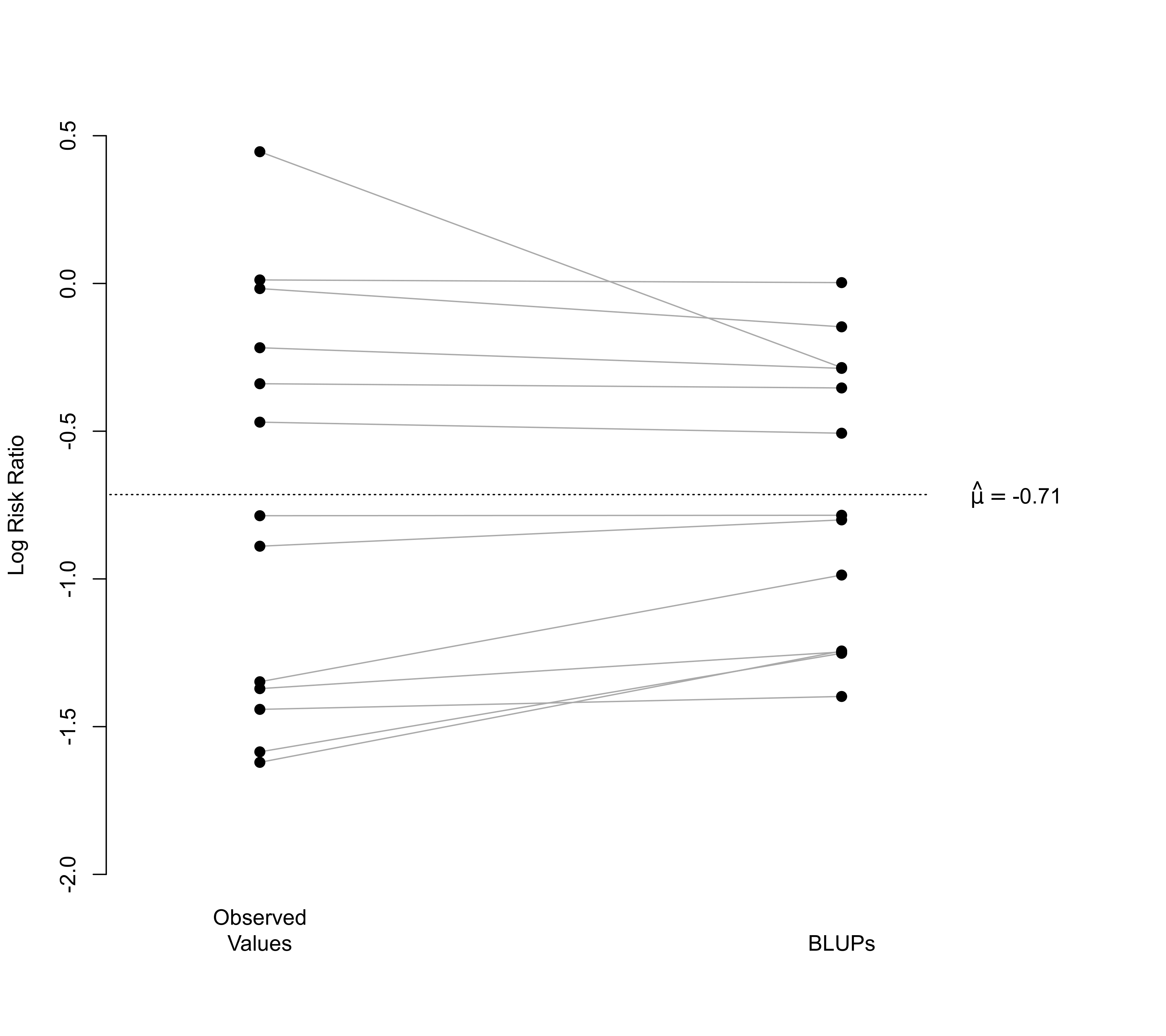
The standard random effects model assumes \(y_i | \theta_i \sim N(\theta_i, v_i)\) and \(\theta_i \sim N(\mu, \tau^2)\). So \(\theta_i\) denotes the true effect in the \(i\)th study and \(y_i\) the corresponding observed effect. While \(y_i\) is an estimate of \(\theta_i\), we can use information from the random-effects model to obtain better estimates of the \(\theta_i\) values. These are the so-called best linear unbiased predictions (BLUPs) of the study-specific true effects, also sometimes called shrunken estimates, as they represent a compromise between the observed effect in the \(i\)th study (i.e., \(y_i\)) and the estimated average effect obtained from the random-effects model (i.e., \(\hat{\mu}\)). They can also be regarded as ‘empirical Bayes’ estimates under certain assumptions.

To be precise, it should be noted that the function actually computes empirical BLUPs (eBLUPs), since the predicted values are a function of the estimated value of \(\tau^2\).

By default, a standard normal distribution is used to construct corresponding prediction intervals. When the model was fitted with test="t", test="knha", test="hksj", or test="adhoc", then a t-distribution with \(k-p\) degrees of freedom is used.

Equal-effects models do not contain random study effects. The BLUPs for these models will therefore be equal to the fitted values, that is, those obtained with fitted and predict.

When using the transf argument, the transformation is applied to the predicted values and the corresponding interval bounds. The standard errors are then set equal to NA and are omitted from the printed output.

Author

Wolfgang Viechtbauer (wvb@metafor-project.org, https://www.metafor-project.org).

References

Kackar, R. N., & Harville, D. A. (1981). Unbiasedness of two-stage estimation and prediction procedures for mixed linear models. Communications in Statistics, Theory and Methods, 10(13), 1249–1261. https://doi.org/10.1080/03610928108828108

Raudenbush, S. W., & Bryk, A. S. (1985). Empirical Bayes meta-analysis. Journal of Educational Statistics, 10(2), 75–98. https://doi.org/10.3102/10769986010002075

Robinson, G. K. (1991). That BLUP is a good thing: The estimation of random effects. Statistical Science, 6(1), 15–32. https://doi.org/10.1214/ss/1177011926

van Aert, R. C. M., Schmid, C. H., Svensson, D., & Jackson, D. (2021). Study specific prediction intervals for random-effects meta-analysis: A tutorial. Research Synthesis Methods, 12(4), 429–447. https://doi.org/10.1002/jrsm.1490

Viechtbauer, W. (2010). Conducting meta-analyses in R with the metafor package. Journal of Statistical Software, 36(3), 1–48. https://doi.org/10.18637/jss.v036.i03

Examples

### calculate log risk ratios and corresponding sampling variances
dat <- escalc(measure="RR", ai=tpos, bi=tneg, ci=cpos, di=cneg, data=dat.bcg)

### meta-analysis of the log risk ratios using a random-effects model
res <- rma(yi, vi, data=dat)

### BLUPs of the true risk ratios for each study
blup(res, transf=exp)
#> 
#>      pred  pi.lb  pi.ub 
#> 1  0.4492 0.2012 1.0032 
#> 2  0.2860 0.1431 0.5716 
#> 3  0.3727 0.1590 0.8740 
#> 4  0.2471 0.1887 0.3236 
#> 5  0.7502 0.4958 1.1352 
#> 6  0.4563 0.3883 0.5362 
#> 7  0.2882 0.1400 0.5936 
#> 8  1.0029 0.8871 1.1338 
#> 9  0.6024 0.3911 0.9279 
#> 10 0.2873 0.1775 0.4651 
#> 11 0.7021 0.5665 0.8702 
#> 12 0.7522 0.3064 1.8469 
#> 13 0.8635 0.5359 1.3915 
#> 

### illustrate shrinkage of BLUPs towards the (estimated) population average
res <- rma(yi, vi, data=dat)
blups <- blup(res)$pred
plot(NA, NA, xlim=c(0.8,2.4), ylim=c(-2,0.5), pch=19,
     xaxt="n", bty="n", xlab="", ylab="Log Risk Ratio")
segments(rep(1,13), dat$yi, rep(2,13), blups, col="darkgray")
points(rep(1,13), dat$yi, pch=19)
points(rep(2,13), blups, pch=19)
axis(side=1, at=c(1,2), labels=c("Observed\nValues", "BLUPs"), lwd=0)
segments(0, res$beta, 2.15, res$beta, lty="dotted")
text(2.3, res$beta, substitute(hat(mu)==muhat, list(muhat=round(res$beta[[1]], 2))), cex=1)