Studies to Illustrate Model Checking Methods
dat.viechtbauer2021.RdResults from 20 hypothetical randomized clinical trials examining the effectiveness of a medication for treating some disease.
dat.viechtbauer2021Format
The data frame contains the following columns:
| trial | numeric | trial number |
| nTi | numeric | number of patients in the treatment group |
| nCi | numeric | number of patients in the control group |
| xTi | numeric | number of patients in the treatment group with remission |
| xCi | numeric | number of patients in the control group with remission |
| dose | numeric | dosage of the medication provided to patients in the treatment group (in milligrams per day) |
Details
The dataset was constructed for the purposes of illustrating the model checking and diagnostic methods described in Viechtbauer (2021). The code below provides the results for many of the analyses and plots discussed in the book chapter.
Source
Viechtbauer, W. (2021). Model checking in meta-analysis. In C. H. Schmid, T. Stijnen, & I. R. White (Eds.), Handbook of meta-analysis (pp. 219-254). Boca Raton, FL: CRC Press. https://doi.org/10.1201/9781315119403
Concepts
medicine, odds ratios, outliers, model checks
Examples
### copy data into 'dat' and examine data
dat <- dat.viechtbauer2021
dat
#> trial nTi nCi xTi xCi dose
#> 1 1 66 59 42 24 100
#> 2 2 59 65 42 34 200
#> 3 3 253 257 96 32 250
#> 4 4 137 144 51 44 125
#> 5 5 327 326 47 39 50
#> 6 6 584 588 38 87 25
#> 7 7 526 532 390 323 125
#> 8 8 28 30 10 3 125
#> 9 9 191 201 165 126 125
#> 10 10 86 94 58 39 150
#> 11 11 229 221 72 60 100
#> 12 12 153 144 79 56 150
#> 13 13 93 95 48 35 200
#> 14 14 40 40 8 4 25
#> 15 15 85 88 44 21 175
#> 16 16 100 107 10 13 25
#> 17 17 72 64 11 9 25
#> 18 18 80 74 47 23 200
#> 19 19 191 195 144 116 100
#> 20 20 85 85 48 49 75
### load metafor package
library(metafor)
### calculate log odds ratios and corresponding sampling variances
dat <- escalc(measure="OR", ai=xTi, n1i=nTi, ci=xCi, n2i=nCi, add=1/2, to="all", data=dat)
dat
#>
#> trial nTi nCi xTi xCi dose yi vi
#> 1 1 66 59 42 24 100 0.9217 0.1333
#> 2 2 59 65 42 34 200 0.7963 0.1414
#> 3 3 253 257 96 32 250 1.4472 0.0519
#> 4 4 137 144 51 44 125 0.2961 0.0634
#> 5 5 327 326 47 39 50 0.2091 0.0534
#> 6 6 584 588 38 87 25 -0.9069 0.0412
#> 7 7 526 532 390 323 125 0.6166 0.0178
#> 8 8 28 30 10 3 125 1.4950 0.4714
#> 9 9 191 201 165 126 125 1.3157 0.0649
#> 10 10 86 94 58 39 150 1.0592 0.0955
#> 11 11 229 221 72 60 100 0.2060 0.0429
#> 12 12 153 144 79 56 150 0.5137 0.0550
#> 13 13 93 95 48 35 200 0.5970 0.0873
#> 14 14 40 40 8 4 25 0.7521 0.3980
#> 15 15 85 88 44 21 175 1.2139 0.1079
#> 16 16 100 107 10 13 25 -0.2081 0.1909
#> 17 17 72 64 11 9 25 0.0884 0.2265
#> 18 18 80 74 47 23 200 1.1338 0.1129
#> 19 19 191 195 144 116 100 0.7304 0.0491
#> 20 20 85 85 48 49 75 -0.0474 0.0949
#>
### number of studies
k <- nrow(dat)
### fit models
res.CE <- rma(yi, vi, data=dat, method="CE") # same as method="EE"
res.CE
#>
#> Common-Effects Model (k = 20)
#>
#> I^2 (total heterogeneity / total variability): 81.70%
#> H^2 (total variability / sampling variability): 5.46
#>
#> Test for Heterogeneity:
#> Q(df = 19) = 103.8068, p-val < .0001
#>
#> Model Results:
#>
#> estimate se zval pval ci.lb ci.ub
#> 0.5295 0.0586 9.0328 <.0001 0.4146 0.6443 ***
#>
#> ---
#> Signif. codes: 0 ‘***’ 0.001 ‘**’ 0.01 ‘*’ 0.05 ‘.’ 0.1 ‘ ’ 1
#>
res.RE <- rma(yi, vi, data=dat, method="DL")
res.RE
#>
#> Random-Effects Model (k = 20; tau^2 estimator: DL)
#>
#> tau^2 (estimated amount of total heterogeneity): 0.3174 (SE = 0.1472)
#> tau (square root of estimated tau^2 value): 0.5634
#> I^2 (total heterogeneity / total variability): 81.70%
#> H^2 (total variability / sampling variability): 5.46
#>
#> Test for Heterogeneity:
#> Q(df = 19) = 103.8068, p-val < .0001
#>
#> Model Results:
#>
#> estimate se zval pval ci.lb ci.ub
#> 0.5867 0.1451 4.0425 <.0001 0.3022 0.8712 ***
#>
#> ---
#> Signif. codes: 0 ‘***’ 0.001 ‘**’ 0.01 ‘*’ 0.05 ‘.’ 0.1 ‘ ’ 1
#>
res.MR <- rma(yi, vi, mods = ~ dose, data=dat, method="FE")
res.MR
#>
#> Fixed-Effects with Moderators Model (k = 20)
#>
#> I^2 (residual heterogeneity / unaccounted variability): 55.49%
#> H^2 (unaccounted variability / sampling variability): 2.25
#> R^2 (amount of heterogeneity accounted for): 58.88%
#>
#> Test for Residual Heterogeneity:
#> QE(df = 18) = 40.4392, p-val = 0.0018
#>
#> Test of Moderators (coefficient 2):
#> QM(df = 1) = 63.3676, p-val < .0001
#>
#> Model Results:
#>
#> estimate se zval pval ci.lb ci.ub
#> intrcpt -0.4235 0.1333 -3.1772 0.0015 -0.6847 -0.1622 **
#> dose 0.0079 0.0010 7.9604 <.0001 0.0059 0.0098 ***
#>
#> ---
#> Signif. codes: 0 ‘***’ 0.001 ‘**’ 0.01 ‘*’ 0.05 ‘.’ 0.1 ‘ ’ 1
#>
res.ME <- rma(yi, vi, mods = ~ dose, data=dat, method="DL")
res.ME
#>
#> Mixed-Effects Model (k = 20; tau^2 estimator: DL)
#>
#> tau^2 (estimated amount of residual heterogeneity): 0.0895 (SE = 0.0582)
#> tau (square root of estimated tau^2 value): 0.2992
#> I^2 (residual heterogeneity / unaccounted variability): 55.49%
#> H^2 (unaccounted variability / sampling variability): 2.25
#> R^2 (amount of heterogeneity accounted for): 71.80%
#>
#> Test for Residual Heterogeneity:
#> QE(df = 18) = 40.4392, p-val = 0.0018
#>
#> Test of Moderators (coefficient 2):
#> QM(df = 1) = 22.6429, p-val < .0001
#>
#> Model Results:
#>
#> estimate se zval pval ci.lb ci.ub
#> intrcpt -0.3041 0.2061 -1.4758 0.1400 -0.7080 0.0998
#> dose 0.0071 0.0015 4.7585 <.0001 0.0042 0.0101 ***
#>
#> ---
#> Signif. codes: 0 ‘***’ 0.001 ‘**’ 0.01 ‘*’ 0.05 ‘.’ 0.1 ‘ ’ 1
#>
### forest and bubble plot
par(mar=c(5,4,1,2))
forest(dat$yi, dat$vi, psize=0.8, efac=0, xlim=c(-4,6), ylim=c(-3,23),
cex=1, width=c(5,5,5), xlab="Log Odds Ratio (LnOR)",
header=c("Trial", "LnOR [95% CI]"))
addpoly(res.CE, row=-1, mlab="CE Model")
addpoly(res.RE, row=-2, mlab="RE Model")
abline(h=0)
 tmp <- regplot(res.ME, xlim=c(0,250), ylim=c(-1,1.5), predlim=c(0,250), shade=FALSE, digits=1,
xlab="Dosage (mg per day)", psize="seinv", plim=c(NA,5), bty="l", las=1,
lty=c("solid", "dashed"), label=TRUE, labsize=0.8, offset=c(1,0.7))
res.sub <- rma(yi, vi, mods = ~ dose, data=dat, method="DL", subset=-6)
abline(res.sub, lty="dotted")
points(tmp$xi, tmp$yi, pch=21, cex=tmp$psize, col="black", bg="darkgray")
tmp <- regplot(res.ME, xlim=c(0,250), ylim=c(-1,1.5), predlim=c(0,250), shade=FALSE, digits=1,
xlab="Dosage (mg per day)", psize="seinv", plim=c(NA,5), bty="l", las=1,
lty=c("solid", "dashed"), label=TRUE, labsize=0.8, offset=c(1,0.7))
res.sub <- rma(yi, vi, mods = ~ dose, data=dat, method="DL", subset=-6)
abline(res.sub, lty="dotted")
points(tmp$xi, tmp$yi, pch=21, cex=tmp$psize, col="black", bg="darkgray")
 par(mar=c(5,4,4,2))
### number of standardized deleted residuals larger than +-1.96 in each model
sum(abs(rstudent(res.CE)$z) >= qnorm(0.975))
#> [1] 4
sum(abs(rstudent(res.MR)$z) >= qnorm(0.975))
#> [1] 3
sum(abs(rstudent(res.RE)$z) >= qnorm(0.975))
#> [1] 1
sum(abs(rstudent(res.ME)$z) >= qnorm(0.975))
#> [1] 2
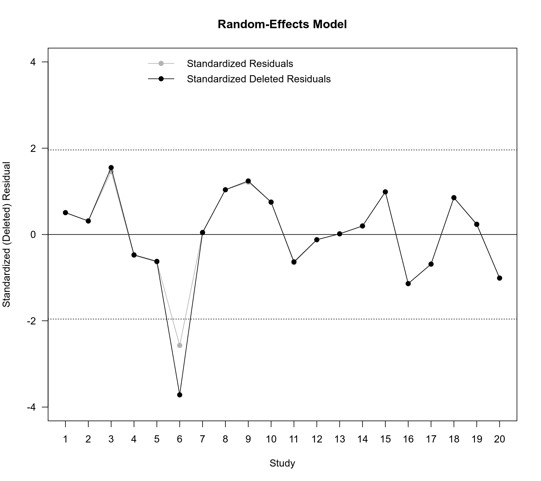
### plot of the standardized deleted residuals for the RE and ME models
plot(NA, NA, xlim=c(1,20), ylim=c(-4,4), xlab="Study", ylab="Standardized (Deleted) Residual",
xaxt="n", main="Random-Effects Model", las=1)
axis(side=1, at=1:20)
abline(h=c(-1.96,1.96), lty="dotted")
abline(h=0)
points(1:20, rstandard(res.RE)$z, type="o", pch=19, col="gray70")
points(1:20, rstudent(res.RE)$z, type="o", pch=19)
legend("top", pch=19, col=c("gray70","black"), lty="solid",
legend=c("Standardized Residuals","Standardized Deleted Residuals"), bty="n")
par(mar=c(5,4,4,2))
### number of standardized deleted residuals larger than +-1.96 in each model
sum(abs(rstudent(res.CE)$z) >= qnorm(0.975))
#> [1] 4
sum(abs(rstudent(res.MR)$z) >= qnorm(0.975))
#> [1] 3
sum(abs(rstudent(res.RE)$z) >= qnorm(0.975))
#> [1] 1
sum(abs(rstudent(res.ME)$z) >= qnorm(0.975))
#> [1] 2
### plot of the standardized deleted residuals for the RE and ME models
plot(NA, NA, xlim=c(1,20), ylim=c(-4,4), xlab="Study", ylab="Standardized (Deleted) Residual",
xaxt="n", main="Random-Effects Model", las=1)
axis(side=1, at=1:20)
abline(h=c(-1.96,1.96), lty="dotted")
abline(h=0)
points(1:20, rstandard(res.RE)$z, type="o", pch=19, col="gray70")
points(1:20, rstudent(res.RE)$z, type="o", pch=19)
legend("top", pch=19, col=c("gray70","black"), lty="solid",
legend=c("Standardized Residuals","Standardized Deleted Residuals"), bty="n")
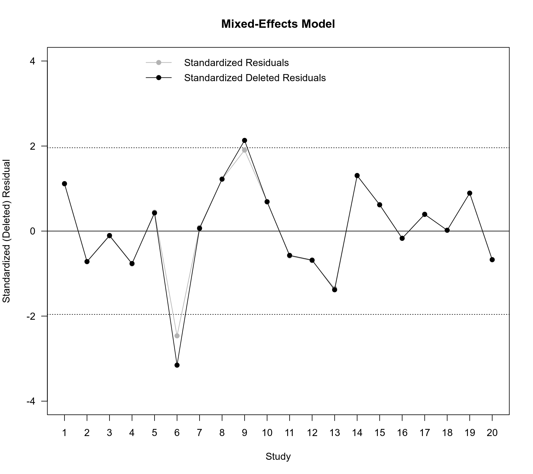
 plot(NA, NA, xlim=c(1,20), ylim=c(-4,4), xlab="Study", ylab="Standardized (Deleted) Residual",
xaxt="n", main="Mixed-Effects Model", las=1)
axis(side=1, at=1:20)
abline(h=c(-1.96,1.96), lty="dotted")
abline(h=0)
points(1:20, rstandard(res.ME)$z, type="o", pch=19, col="gray70")
points(1:20, rstudent(res.ME)$z, type="o", pch=19)
legend("top", pch=19, col=c("gray70","black"), lty="solid",
legend=c("Standardized Residuals","Standardized Deleted Residuals"), bty="n")
plot(NA, NA, xlim=c(1,20), ylim=c(-4,4), xlab="Study", ylab="Standardized (Deleted) Residual",
xaxt="n", main="Mixed-Effects Model", las=1)
axis(side=1, at=1:20)
abline(h=c(-1.96,1.96), lty="dotted")
abline(h=0)
points(1:20, rstandard(res.ME)$z, type="o", pch=19, col="gray70")
points(1:20, rstudent(res.ME)$z, type="o", pch=19)
legend("top", pch=19, col=c("gray70","black"), lty="solid",
legend=c("Standardized Residuals","Standardized Deleted Residuals"), bty="n")
 ### Baujat plots
baujat(res.CE, main="Common-Effects Model", xlab="Squared Pearson Residual", ylim=c(0,5), las=1)
### Baujat plots
baujat(res.CE, main="Common-Effects Model", xlab="Squared Pearson Residual", ylim=c(0,5), las=1)
 baujat(res.ME, main="Mixed-Effects Model", ylim=c(0,2), las=1)
 ### GOSH plots (skipped because this takes quite some time to run)
if (FALSE) {
res.GOSH.CE <- gosh(res.CE, subsets=10^7)
plot(res.GOSH.CE, cex=0.2, out=6, xlim=c(-0.25,1.25), breaks=c(200,100))
res.GOSH.ME <- gosh(res.ME, subsets=10^7)
plot(res.GOSH.ME, het="tau2", out=6, breaks=50, adjust=0.6, las=1)
}
### plot of treatment dosage against the standardized residuals
plot(dat$dose, rstandard(res.ME)$z, pch=19, xlab="Dosage (mg per day)",
ylab="Standardized Residual", xlim=c(0,250), ylim=c(-2.5,2.5), las=1)
abline(h=c(-1.96,1.96), lty="dotted", lwd=2)
abline(h=0)
title("Standardized Residual Plot")
text(dat$dose[6], rstandard(res.ME)$z[6], "6", pos=4, offset=0.4)
### GOSH plots (skipped because this takes quite some time to run)
if (FALSE) {
res.GOSH.CE <- gosh(res.CE, subsets=10^7)
plot(res.GOSH.CE, cex=0.2, out=6, xlim=c(-0.25,1.25), breaks=c(200,100))
res.GOSH.ME <- gosh(res.ME, subsets=10^7)
plot(res.GOSH.ME, het="tau2", out=6, breaks=50, adjust=0.6, las=1)
}
### plot of treatment dosage against the standardized residuals
plot(dat$dose, rstandard(res.ME)$z, pch=19, xlab="Dosage (mg per day)",
ylab="Standardized Residual", xlim=c(0,250), ylim=c(-2.5,2.5), las=1)
abline(h=c(-1.96,1.96), lty="dotted", lwd=2)
abline(h=0)
title("Standardized Residual Plot")
text(dat$dose[6], rstandard(res.ME)$z[6], "6", pos=4, offset=0.4)
 ### quadratic polynomial model
rma(yi, vi, mods = ~ dose + I(dose^2), data=dat, method="DL")
#>
#> Mixed-Effects Model (k = 20; tau^2 estimator: DL)
#>
#> tau^2 (estimated amount of residual heterogeneity): 0.0807 (SE = 0.0568)
#> tau (square root of estimated tau^2 value): 0.2840
#> I^2 (residual heterogeneity / unaccounted variability): 52.00%
#> H^2 (unaccounted variability / sampling variability): 2.08
#> R^2 (amount of heterogeneity accounted for): 74.58%
#>
#> Test for Residual Heterogeneity:
#> QE(df = 17) = 35.4193, p-val = 0.0055
#>
#> Test of Moderators (coefficients 2:3):
#> QM(df = 2) = 25.7249, p-val < .0001
#>
#> Model Results:
#>
#> estimate se zval pval ci.lb ci.ub
#> intrcpt -0.6191 0.3163 -1.9571 0.0503 -1.2390 0.0009 .
#> dose 0.0136 0.0053 2.5694 0.0102 0.0032 0.0240 *
#> I(dose^2) -0.0000 0.0000 -1.2610 0.2073 -0.0001 0.0000
#>
#> ---
#> Signif. codes: 0 ‘***’ 0.001 ‘**’ 0.01 ‘*’ 0.05 ‘.’ 0.1 ‘ ’ 1
#>
### lack-of-fit model
resLOF <- rma(yi, vi, mods = ~ dose + factor(dose), data=dat, method="DL", btt=3:9)
#> Warning: Redundant predictors dropped from the model.
resLOF
#>
#> Mixed-Effects Model (k = 20; tau^2 estimator: DL)
#>
#> tau^2 (estimated amount of residual heterogeneity): 0.1285 (SE = 0.0981)
#> tau (square root of estimated tau^2 value): 0.3585
#> I^2 (residual heterogeneity / unaccounted variability): 60.32%
#> H^2 (unaccounted variability / sampling variability): 2.52
#> R^2 (amount of heterogeneity accounted for): 59.50%
#>
#> Test for Residual Heterogeneity:
#> QE(df = 11) = 27.7226, p-val = 0.0036
#>
#> Test of Moderators (coefficients 3:9):
#> QM(df = 7) = 3.5712, p-val = 0.8276
#>
#> Model Results:
#>
#> estimate se zval pval ci.lb ci.ub
#> intrcpt -0.5099 0.3035 -1.6803 0.0929 -1.1048 0.0849 .
#> dose 0.0078 0.0022 3.5002 0.0005 0.0034 0.0122 ***
#> factor(dose)50 0.3276 0.4916 0.6663 0.5052 -0.6360 1.2912
#> factor(dose)75 -0.1246 0.5257 -0.2371 0.8126 -1.1550 0.9057
#> factor(dose)100 0.3051 0.3433 0.8887 0.3741 -0.3677 0.9779
#> factor(dose)125 0.3285 0.3333 0.9856 0.3243 -0.3247 0.9817
#> factor(dose)150 0.0950 0.4135 0.2298 0.8183 -0.7154 0.9054
#> factor(dose)175 0.3538 0.5698 0.6209 0.5347 -0.7631 1.4707
#> factor(dose)200 -0.2215 0.4392 -0.5042 0.6141 -1.0822 0.6393
#>
#> ---
#> Signif. codes: 0 ‘***’ 0.001 ‘**’ 0.01 ‘*’ 0.05 ‘.’ 0.1 ‘ ’ 1
#>
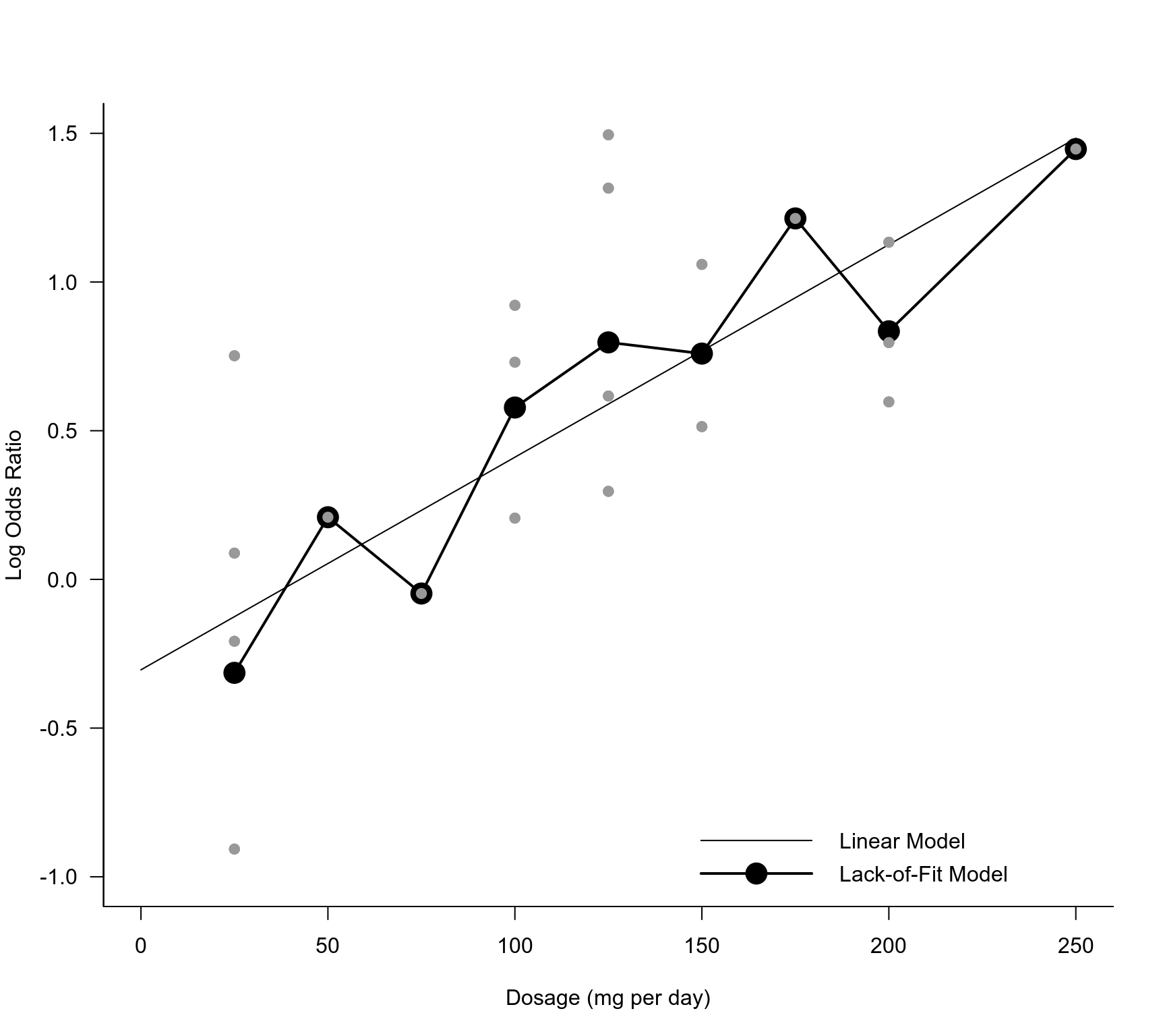
### scatter plot to illustrate the lack-of-fit model
regplot(res.ME, xlim=c(0,250), ylim=c(-1.0,1.5), xlab="Dosage (mg per day)", ci=FALSE,
predlim=c(0,250), psize=1, pch=19, col="gray60", digits=1, lwd=1, bty="l", las=1)
dosages <- sort(unique(dat$dose))
lines(dosages, fitted(resLOF)[match(dosages, dat$dose)], type="o", pch=19, cex=2, lwd=2)
points(dat$dose, dat$yi, pch=19, col="gray60")
legend("bottomright", legend=c("Linear Model", "Lack-of-Fit Model"), pch=c(NA,19), col="black",
lty="solid", lwd=c(1,2), pt.cex=c(1,2), seg.len=4, bty="n")
### quadratic polynomial model
rma(yi, vi, mods = ~ dose + I(dose^2), data=dat, method="DL")
#>
#> Mixed-Effects Model (k = 20; tau^2 estimator: DL)
#>
#> tau^2 (estimated amount of residual heterogeneity): 0.0807 (SE = 0.0568)
#> tau (square root of estimated tau^2 value): 0.2840
#> I^2 (residual heterogeneity / unaccounted variability): 52.00%
#> H^2 (unaccounted variability / sampling variability): 2.08
#> R^2 (amount of heterogeneity accounted for): 74.58%
#>
#> Test for Residual Heterogeneity:
#> QE(df = 17) = 35.4193, p-val = 0.0055
#>
#> Test of Moderators (coefficients 2:3):
#> QM(df = 2) = 25.7249, p-val < .0001
#>
#> Model Results:
#>
#> estimate se zval pval ci.lb ci.ub
#> intrcpt -0.6191 0.3163 -1.9571 0.0503 -1.2390 0.0009 .
#> dose 0.0136 0.0053 2.5694 0.0102 0.0032 0.0240 *
#> I(dose^2) -0.0000 0.0000 -1.2610 0.2073 -0.0001 0.0000
#>
#> ---
#> Signif. codes: 0 ‘***’ 0.001 ‘**’ 0.01 ‘*’ 0.05 ‘.’ 0.1 ‘ ’ 1
#>
### lack-of-fit model
resLOF <- rma(yi, vi, mods = ~ dose + factor(dose), data=dat, method="DL", btt=3:9)
#> Warning: Redundant predictors dropped from the model.
resLOF
#>
#> Mixed-Effects Model (k = 20; tau^2 estimator: DL)
#>
#> tau^2 (estimated amount of residual heterogeneity): 0.1285 (SE = 0.0981)
#> tau (square root of estimated tau^2 value): 0.3585
#> I^2 (residual heterogeneity / unaccounted variability): 60.32%
#> H^2 (unaccounted variability / sampling variability): 2.52
#> R^2 (amount of heterogeneity accounted for): 59.50%
#>
#> Test for Residual Heterogeneity:
#> QE(df = 11) = 27.7226, p-val = 0.0036
#>
#> Test of Moderators (coefficients 3:9):
#> QM(df = 7) = 3.5712, p-val = 0.8276
#>
#> Model Results:
#>
#> estimate se zval pval ci.lb ci.ub
#> intrcpt -0.5099 0.3035 -1.6803 0.0929 -1.1048 0.0849 .
#> dose 0.0078 0.0022 3.5002 0.0005 0.0034 0.0122 ***
#> factor(dose)50 0.3276 0.4916 0.6663 0.5052 -0.6360 1.2912
#> factor(dose)75 -0.1246 0.5257 -0.2371 0.8126 -1.1550 0.9057
#> factor(dose)100 0.3051 0.3433 0.8887 0.3741 -0.3677 0.9779
#> factor(dose)125 0.3285 0.3333 0.9856 0.3243 -0.3247 0.9817
#> factor(dose)150 0.0950 0.4135 0.2298 0.8183 -0.7154 0.9054
#> factor(dose)175 0.3538 0.5698 0.6209 0.5347 -0.7631 1.4707
#> factor(dose)200 -0.2215 0.4392 -0.5042 0.6141 -1.0822 0.6393
#>
#> ---
#> Signif. codes: 0 ‘***’ 0.001 ‘**’ 0.01 ‘*’ 0.05 ‘.’ 0.1 ‘ ’ 1
#>
### scatter plot to illustrate the lack-of-fit model
regplot(res.ME, xlim=c(0,250), ylim=c(-1.0,1.5), xlab="Dosage (mg per day)", ci=FALSE,
predlim=c(0,250), psize=1, pch=19, col="gray60", digits=1, lwd=1, bty="l", las=1)
dosages <- sort(unique(dat$dose))
lines(dosages, fitted(resLOF)[match(dosages, dat$dose)], type="o", pch=19, cex=2, lwd=2)
points(dat$dose, dat$yi, pch=19, col="gray60")
legend("bottomright", legend=c("Linear Model", "Lack-of-Fit Model"), pch=c(NA,19), col="black",
lty="solid", lwd=c(1,2), pt.cex=c(1,2), seg.len=4, bty="n")
 ### checking normality of the standardized deleted residuals
qqnorm(res.ME, type="rstudent", main="Standardized Deleted Residuals", pch=19, label="out",
lwd=2, pos=24, ylim=c(-4,3), lty=c("solid", "dotted"), las=1)
### checking normality of the standardized deleted residuals
qqnorm(res.ME, type="rstudent", main="Standardized Deleted Residuals", pch=19, label="out",
lwd=2, pos=24, ylim=c(-4,3), lty=c("solid", "dotted"), las=1)
 ### checking normality of the random effects
sav <- qqnorm(ranef(res.ME)$pred, main="BLUPs of the Random Effects", cex=1, pch=19,
xlim=c(-2.2,2.2), ylim=c(-0.6,0.6), las=1)
abline(a=0, b=sd(ranef(res.ME)$pred), lwd=2)
text(sav$x[6], sav$y[6], "6", pos=4, offset=0.4)
### checking normality of the random effects
sav <- qqnorm(ranef(res.ME)$pred, main="BLUPs of the Random Effects", cex=1, pch=19,
xlim=c(-2.2,2.2), ylim=c(-0.6,0.6), las=1)
abline(a=0, b=sd(ranef(res.ME)$pred), lwd=2)
text(sav$x[6], sav$y[6], "6", pos=4, offset=0.4)
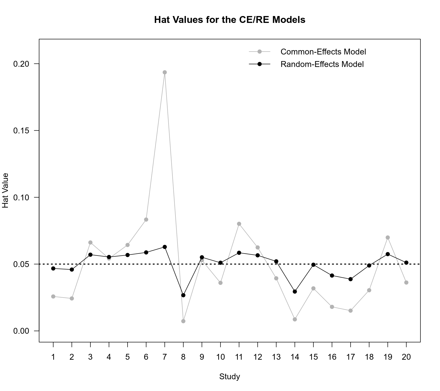
 ### hat values for the CE and RE models
plot(NA, NA, xlim=c(1,20), ylim=c(0,0.21), xaxt="n", las=1, xlab="Study", ylab="Hat Value")
axis(1, 1:20, cex.axis=1)
points(hatvalues(res.CE), type="o", pch=19, col="gray70")
points(hatvalues(res.RE), type="o", pch=19)
abline(h=1/20, lty="dotted", lwd=2)
title("Hat Values for the CE/RE Models")
legend("topright", pch=19, col=c("gray70","black"), lty="solid",
legend=c("Common-Effects Model", "Random-Effects Model"), bty="n")
### hat values for the CE and RE models
plot(NA, NA, xlim=c(1,20), ylim=c(0,0.21), xaxt="n", las=1, xlab="Study", ylab="Hat Value")
axis(1, 1:20, cex.axis=1)
points(hatvalues(res.CE), type="o", pch=19, col="gray70")
points(hatvalues(res.RE), type="o", pch=19)
abline(h=1/20, lty="dotted", lwd=2)
title("Hat Values for the CE/RE Models")
legend("topright", pch=19, col=c("gray70","black"), lty="solid",
legend=c("Common-Effects Model", "Random-Effects Model"), bty="n")
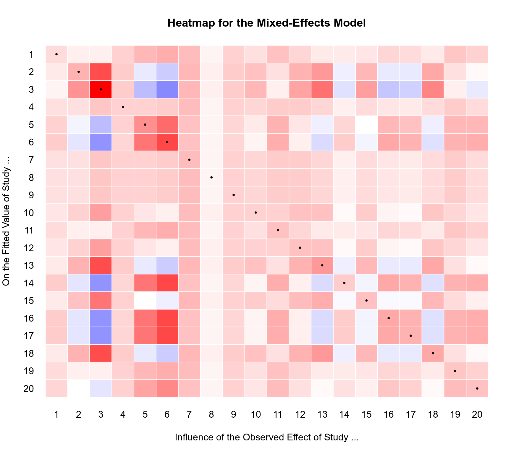
 ### heatmap of the hat matrix for the ME model
cols <- colorRampPalette(c("blue", "white", "red"))(101)
h <- hatvalues(res.ME, type="matrix")
image(1:nrow(h), 1:ncol(h), t(h[nrow(h):1,]), axes=FALSE,
xlab="Influence of the Observed Effect of Study ...", ylab="On the Fitted Value of Study ...",
col=cols, zlim=c(-max(abs(h)),max(abs(h))))
axis(1, 1:20, tick=FALSE)
axis(2, 1:20, labels=20:1, las=1, tick=FALSE)
abline(h=seq(0.5,20.5,by=1), col="white")
abline(v=seq(0.5,20.5,by=1), col="white")
points(1:20, 20:1, pch=19, cex=0.4)
title("Heatmap for the Mixed-Effects Model")
### heatmap of the hat matrix for the ME model
cols <- colorRampPalette(c("blue", "white", "red"))(101)
h <- hatvalues(res.ME, type="matrix")
image(1:nrow(h), 1:ncol(h), t(h[nrow(h):1,]), axes=FALSE,
xlab="Influence of the Observed Effect of Study ...", ylab="On the Fitted Value of Study ...",
col=cols, zlim=c(-max(abs(h)),max(abs(h))))
axis(1, 1:20, tick=FALSE)
axis(2, 1:20, labels=20:1, las=1, tick=FALSE)
abline(h=seq(0.5,20.5,by=1), col="white")
abline(v=seq(0.5,20.5,by=1), col="white")
points(1:20, 20:1, pch=19, cex=0.4)
title("Heatmap for the Mixed-Effects Model")
 ### plot of leverages versus standardized residuals for the ME model
plot(hatvalues(res.ME), rstudent(res.ME)$z, pch=19, cex=0.2+3*sqrt(cooks.distance(res.ME)),
las=1, xlab="Leverage (Hat Value)", ylab="Standardized Deleted Residual",
xlim=c(0,0.35), ylim=c(-3.5,2.5))
abline(h=c(-1.96,1.96), lty="dotted", lwd=2)
abline(h=0, lwd=2)
ids <- c(3,6,9)
text(hatvalues(res.ME)[ids] + c(0,0.013,0.010), rstudent(res.ME)$z[ids] - c(0.18,0,0), ids)
title("Leverage vs. Standardized Deleted Residuals")
### plot of leverages versus standardized residuals for the ME model
plot(hatvalues(res.ME), rstudent(res.ME)$z, pch=19, cex=0.2+3*sqrt(cooks.distance(res.ME)),
las=1, xlab="Leverage (Hat Value)", ylab="Standardized Deleted Residual",
xlim=c(0,0.35), ylim=c(-3.5,2.5))
abline(h=c(-1.96,1.96), lty="dotted", lwd=2)
abline(h=0, lwd=2)
ids <- c(3,6,9)
text(hatvalues(res.ME)[ids] + c(0,0.013,0.010), rstudent(res.ME)$z[ids] - c(0.18,0,0), ids)
title("Leverage vs. Standardized Deleted Residuals")
 ### plot of the Cook's distances for the ME model
plot(1:20, cooks.distance(res.ME), ylim=c(0,1.6), type="o", pch=19, las=1, xaxt="n", yaxt="n",
xlab="Study", ylab="Cook's Distance")
axis(1, 1:20, cex.axis=1)
axis(2, seq(0,1.6,by=0.4), las=1)
title("Cook's Distances")
### plot of the Cook's distances for the ME model
plot(1:20, cooks.distance(res.ME), ylim=c(0,1.6), type="o", pch=19, las=1, xaxt="n", yaxt="n",
xlab="Study", ylab="Cook's Distance")
axis(1, 1:20, cex.axis=1)
axis(2, seq(0,1.6,by=0.4), las=1)
title("Cook's Distances")
 ### plot of the leave-one-out estimates of tau^2 for the ME model
x <- influence(res.ME)
plot(1:20, x$inf$tau2.del, ylim=c(0,0.15), type="o", pch=19, las=1, xaxt="n", xlab="Study",
ylab=expression(paste("Estimate of ", tau^2, " without the ", italic(i), "th study")))
abline(h=res.ME$tau2, lty="dashed")
axis(1, 1:20)
title("Residual Heterogeneity Estimates")
### plot of the leave-one-out estimates of tau^2 for the ME model
x <- influence(res.ME)
plot(1:20, x$inf$tau2.del, ylim=c(0,0.15), type="o", pch=19, las=1, xaxt="n", xlab="Study",
ylab=expression(paste("Estimate of ", tau^2, " without the ", italic(i), "th study")))
abline(h=res.ME$tau2, lty="dashed")
axis(1, 1:20)
title("Residual Heterogeneity Estimates")
 ### plot of the covariance ratios for the ME model
plot(1:20, x$inf$cov.r, ylim=c(0,2.0), type="o", pch=19, las=1, xaxt="n",
xlab="Study", ylab="Covariance Ratio")
abline(h=1, lty="dashed")
axis(1, 1:20)
title("Covariance Ratios")
### plot of the covariance ratios for the ME model
plot(1:20, x$inf$cov.r, ylim=c(0,2.0), type="o", pch=19, las=1, xaxt="n",
xlab="Study", ylab="Covariance Ratio")
abline(h=1, lty="dashed")
axis(1, 1:20)
title("Covariance Ratios")
 ### fit mixed-effects model without studies 3 and/or 6
rma(yi, vi, mods = ~ dose, data=dat, method="DL", subset=-3)
#>
#> Mixed-Effects Model (k = 19; tau^2 estimator: DL)
#>
#> tau^2 (estimated amount of residual heterogeneity): 0.0994 (SE = 0.0645)
#> tau (square root of estimated tau^2 value): 0.3153
#> I^2 (residual heterogeneity / unaccounted variability): 57.63%
#> H^2 (unaccounted variability / sampling variability): 2.36
#> R^2 (amount of heterogeneity accounted for): 64.04%
#>
#> Test for Residual Heterogeneity:
#> QE(df = 17) = 40.1225, p-val = 0.0012
#>
#> Test of Moderators (coefficient 2):
#> QM(df = 1) = 15.7509, p-val < .0001
#>
#> Model Results:
#>
#> estimate se zval pval ci.lb ci.ub
#> intrcpt -0.3064 0.2290 -1.3381 0.1809 -0.7553 0.1424
#> dose 0.0072 0.0018 3.9687 <.0001 0.0037 0.0108 ***
#>
#> ---
#> Signif. codes: 0 ‘***’ 0.001 ‘**’ 0.01 ‘*’ 0.05 ‘.’ 0.1 ‘ ’ 1
#>
rma(yi, vi, mods = ~ dose, data=dat, method="DL", subset=-6)
#>
#> Mixed-Effects Model (k = 19; tau^2 estimator: DL)
#>
#> tau^2 (estimated amount of residual heterogeneity): 0.0321 (SE = 0.0375)
#> tau (square root of estimated tau^2 value): 0.1792
#> I^2 (residual heterogeneity / unaccounted variability): 30.17%
#> H^2 (unaccounted variability / sampling variability): 1.43
#> R^2 (amount of heterogeneity accounted for): 75.00%
#>
#> Test for Residual Heterogeneity:
#> QE(df = 17) = 24.3434, p-val = 0.1104
#>
#> Test of Moderators (coefficient 2):
#> QM(df = 1) = 16.7472, p-val < .0001
#>
#> Model Results:
#>
#> estimate se zval pval ci.lb ci.ub
#> intrcpt -0.0504 0.1926 -0.2615 0.7937 -0.4279 0.3272
#> dose 0.0056 0.0014 4.0923 <.0001 0.0029 0.0082 ***
#>
#> ---
#> Signif. codes: 0 ‘***’ 0.001 ‘**’ 0.01 ‘*’ 0.05 ‘.’ 0.1 ‘ ’ 1
#>
rma(yi, vi, mods = ~ dose, data=dat, method="DL", subset=-c(3,6))
#>
#> Mixed-Effects Model (k = 18; tau^2 estimator: DL)
#>
#> tau^2 (estimated amount of residual heterogeneity): 0.0375 (SE = 0.0412)
#> tau (square root of estimated tau^2 value): 0.1937
#> I^2 (residual heterogeneity / unaccounted variability): 33.24%
#> H^2 (unaccounted variability / sampling variability): 1.50
#> R^2 (amount of heterogeneity accounted for): 56.68%
#>
#> Test for Residual Heterogeneity:
#> QE(df = 16) = 23.9677, p-val = 0.0902
#>
#> Test of Moderators (coefficient 2):
#> QM(df = 1) = 8.8711, p-val = 0.0029
#>
#> Model Results:
#>
#> estimate se zval pval ci.lb ci.ub
#> intrcpt -0.0007 0.2216 -0.0030 0.9976 -0.4350 0.4337
#> dose 0.0051 0.0017 2.9784 0.0029 0.0017 0.0084 **
#>
#> ---
#> Signif. codes: 0 ‘***’ 0.001 ‘**’ 0.01 ‘*’ 0.05 ‘.’ 0.1 ‘ ’ 1
#>
### fit mixed-effects model without studies 3 and/or 6
rma(yi, vi, mods = ~ dose, data=dat, method="DL", subset=-3)
#>
#> Mixed-Effects Model (k = 19; tau^2 estimator: DL)
#>
#> tau^2 (estimated amount of residual heterogeneity): 0.0994 (SE = 0.0645)
#> tau (square root of estimated tau^2 value): 0.3153
#> I^2 (residual heterogeneity / unaccounted variability): 57.63%
#> H^2 (unaccounted variability / sampling variability): 2.36
#> R^2 (amount of heterogeneity accounted for): 64.04%
#>
#> Test for Residual Heterogeneity:
#> QE(df = 17) = 40.1225, p-val = 0.0012
#>
#> Test of Moderators (coefficient 2):
#> QM(df = 1) = 15.7509, p-val < .0001
#>
#> Model Results:
#>
#> estimate se zval pval ci.lb ci.ub
#> intrcpt -0.3064 0.2290 -1.3381 0.1809 -0.7553 0.1424
#> dose 0.0072 0.0018 3.9687 <.0001 0.0037 0.0108 ***
#>
#> ---
#> Signif. codes: 0 ‘***’ 0.001 ‘**’ 0.01 ‘*’ 0.05 ‘.’ 0.1 ‘ ’ 1
#>
rma(yi, vi, mods = ~ dose, data=dat, method="DL", subset=-6)
#>
#> Mixed-Effects Model (k = 19; tau^2 estimator: DL)
#>
#> tau^2 (estimated amount of residual heterogeneity): 0.0321 (SE = 0.0375)
#> tau (square root of estimated tau^2 value): 0.1792
#> I^2 (residual heterogeneity / unaccounted variability): 30.17%
#> H^2 (unaccounted variability / sampling variability): 1.43
#> R^2 (amount of heterogeneity accounted for): 75.00%
#>
#> Test for Residual Heterogeneity:
#> QE(df = 17) = 24.3434, p-val = 0.1104
#>
#> Test of Moderators (coefficient 2):
#> QM(df = 1) = 16.7472, p-val < .0001
#>
#> Model Results:
#>
#> estimate se zval pval ci.lb ci.ub
#> intrcpt -0.0504 0.1926 -0.2615 0.7937 -0.4279 0.3272
#> dose 0.0056 0.0014 4.0923 <.0001 0.0029 0.0082 ***
#>
#> ---
#> Signif. codes: 0 ‘***’ 0.001 ‘**’ 0.01 ‘*’ 0.05 ‘.’ 0.1 ‘ ’ 1
#>
rma(yi, vi, mods = ~ dose, data=dat, method="DL", subset=-c(3,6))
#>
#> Mixed-Effects Model (k = 18; tau^2 estimator: DL)
#>
#> tau^2 (estimated amount of residual heterogeneity): 0.0375 (SE = 0.0412)
#> tau (square root of estimated tau^2 value): 0.1937
#> I^2 (residual heterogeneity / unaccounted variability): 33.24%
#> H^2 (unaccounted variability / sampling variability): 1.50
#> R^2 (amount of heterogeneity accounted for): 56.68%
#>
#> Test for Residual Heterogeneity:
#> QE(df = 16) = 23.9677, p-val = 0.0902
#>
#> Test of Moderators (coefficient 2):
#> QM(df = 1) = 8.8711, p-val = 0.0029
#>
#> Model Results:
#>
#> estimate se zval pval ci.lb ci.ub
#> intrcpt -0.0007 0.2216 -0.0030 0.9976 -0.4350 0.4337
#> dose 0.0051 0.0017 2.9784 0.0029 0.0017 0.0084 **
#>
#> ---
#> Signif. codes: 0 ‘***’ 0.001 ‘**’ 0.01 ‘*’ 0.05 ‘.’ 0.1 ‘ ’ 1
#>