Studies on the Effectiveness of Practice Facilitation Interventions
dat.baskerville2012.RdResults from 23 studies on the effectiveness of practice facilitation interventions within the primary care practice setting.
dat.baskerville2012Format
The data frame contains the following columns:
| author | character | study author(s) |
| year | numeric | publication year |
| score | numeric | quality score (0 to 12 scale) |
| design | character | study design (cct = controlled clinical trial, rct = randomized clinical trial, crct = cluster randomized clinical trial) |
| alloconc | numeric | allocation concealed (0 = no, 1 = yes) |
| blind | numeric | single- or double-blind study (0 = no, 1 = yes) |
| itt | numeric | intention to treat analysis (0 = no, 1 = yes) |
| fumonths | numeric | follow-up months |
| retention | numeric | retention (in percent) |
| country | character | country where study was conducted |
| outcomes | numeric | number of outcomes assessed |
| duration | numeric | duration of intervention |
| pperf | numeric | practices per facilitator |
| meetings | numeric | (average) number of meetings |
| hours | numeric | (average) hours per meeting |
| tailor | numeric | intervention tailored to the context and needs of the practice (0 = no, 1 = yes) |
| smd | numeric | standardized mean difference |
| se | numeric | corresponding standard error |
Details
Baskerville et al. (2012) describe outreach or practice facilitation as a "multifaceted approach that involves skilled individuals who enable others, through a range of intervention components and approaches, to address the challenges in implementing evidence-based care guidelines within the primary care setting". The studies included in this dataset examined the effectiveness of practice facilitation interventions for improving some relevant evidence-based practice behavior. The effect was quantified in terms of a standardized mean difference, comparing the change (from pre- to post-intervention) in the intervention versus the comparison group (or the difference from baseline in prospective cohort studies).
Note
The quality score of 18 given for the study by Deitrich et al. (1992) in Table 1 of Baskerville et al. (2012) appears to be a typo. This was corrected to an 8 in the present dataset.
Source
Baskerville, N. B., Liddy, C., & Hogg, W. (2012). Systematic review and meta-analysis of practice facilitation within primary care settings. Annals of Family Medicine, 10(1), 63–74. https://doi.org/10.1370/afm.1312
Concepts
medicine, primary care, standardized mean differences, publication bias, meta-regression
Examples
### copy data into 'dat' and examine data
dat <- dat.baskerville2012
dat
#> author year score design alloconc blind itt fumonths retention country outcomes duration
#> 1 Kottke et al. 1992 6 cct 0 1 1 19 83.0 US 2 18
#> 2 McBride et al. 2000 6 rct 0 0 0 18 100.0 US 4 12
#> 3 Stange et al. 2000 6 rct 0 0 0 24 NA US 35 12
#> 4 Lobo et al. 2004 6 rct 1 0 0 21 57.0 NL 16 21
#> 5 Roetzhiem et al. 2005 6 crct 0 1 0 24 100.0 US 3 24
#> 6 Hogg et al. 2008 6 cct 0 0 1 6 87.0 Can 26 12
#> 7 Aspy et al. 2008 6 cct 0 1 0 18 89.0 US 4 18
#> 8 Jaen et al. 2010 6 rct 0 1 0 26 86.0 US 11 26
#> 9 Cockburn et al. 1992 7 rct 0 0 0 3 79.0 Aus 2 2
#> 10 Modell et al. 1998 7 rct 0 0 0 12 100.0 UK 1 12
#> 11 Engels et al. 2006 7 rct 1 0 1 12 92.0 NL 7 5
#> 12 Aspy et al. 2008 7 rct 0 1 0 9 100.0 US 1 9
#> 13 Deitrich et al. 1992 8 rct 0 1 0 12 96.0 NL 16 21
#> 14 Lobo et al. 2002 8 rct 1 0 1 21 100.0 US 10 3
#> 15 Bryce et al. 1995 9 rct 1 1 1 12 93.3 US 4 12
#> 16 Kinsinger et al. 1998 9 rct 1 1 0 18 94.0 US 5 12
#> 17 Solberg et al. 1998 9 rct 1 0 1 22 100.0 US 10 22
#> 18 Lemelin et al. 2001 9 rct 1 1 0 18 98.0 Can 13 18
#> 19 Frijling et al. 2002 9 crct 1 1 1 21 95.0 NL 7 21
#> 20 Frijling et al. 2003 9 crct 1 1 1 21 95.0 NL 12 21
#> 21 Margolis et al. 2004 10 rct 1 1 1 30 100.0 US 4 24
#> 22 Mold et al. 2008 10 rct 1 1 1 6 100.0 US 6 6
#> 23 Hogg et al. 2008 12 rct 1 1 1 13 100.0 Can 53 12
#> pperf meetings hours tailor smd se
#> 1 5.5 30.0 1.00 1 1.01 0.52
#> 2 NA 5.0 1.00 1 0.82 0.46
#> 3 20.0 4.0 1.50 1 0.59 0.23
#> 4 5.0 15.0 1.00 1 0.44 0.18
#> 5 4.0 4.0 1.00 0 0.84 0.29
#> 6 11.0 12.0 1.50 1 0.73 0.29
#> 7 3.0 3.0 6.00 1 1.12 0.36
#> 8 6.0 4.5 6.00 1 0.04 0.37
#> 9 40.0 2.0 0.25 0 0.24 0.15
#> 10 13.0 3.0 1.00 0 0.32 0.40
#> 11 NA 5.0 1.00 1 1.04 0.32
#> 12 6.0 18.0 6.00 1 1.31 0.57
#> 13 20.0 15.0 1.00 1 0.59 0.29
#> 14 8.0 3.0 1.00 1 0.66 0.19
#> 15 12.0 1.0 15.00 0 0.62 0.31
#> 16 13.0 10.0 0.75 1 0.47 0.27
#> 17 11.0 4.0 3.00 1 1.08 0.32
#> 18 8.0 33.0 1.75 1 0.98 0.32
#> 19 20.0 15.0 1.00 0 0.26 0.18
#> 20 20.0 15.0 1.00 1 0.39 0.18
#> 21 11.0 9.0 1.00 1 0.60 0.31
#> 22 8.0 18.0 4.00 1 0.94 0.53
#> 23 14.0 9.0 0.75 1 0.11 0.27
### load metafor package
library(metafor)
### random-effects model
res <- rma(smd, sei=se, data=dat, method="DL")
print(res, digits=2)
#>
#> Random-Effects Model (k = 23; tau^2 estimator: DL)
#>
#> tau^2 (estimated amount of total heterogeneity): 0.02 (SE = 0.03)
#> tau (square root of estimated tau^2 value): 0.13
#> I^2 (total heterogeneity / total variability): 20.15%
#> H^2 (total variability / sampling variability): 1.25
#>
#> Test for Heterogeneity:
#> Q(df = 22) = 27.55, p-val = 0.19
#>
#> Model Results:
#>
#> estimate se zval pval ci.lb ci.ub
#> 0.56 0.06 8.70 <.01 0.43 0.68 ***
#>
#> ---
#> Signif. codes: 0 ‘***’ 0.001 ‘**’ 0.01 ‘*’ 0.05 ‘.’ 0.1 ‘ ’ 1
#>
### funnel plot
funnel(res, xlab="Standardized Mean Difference", ylim=c(0,0.6))
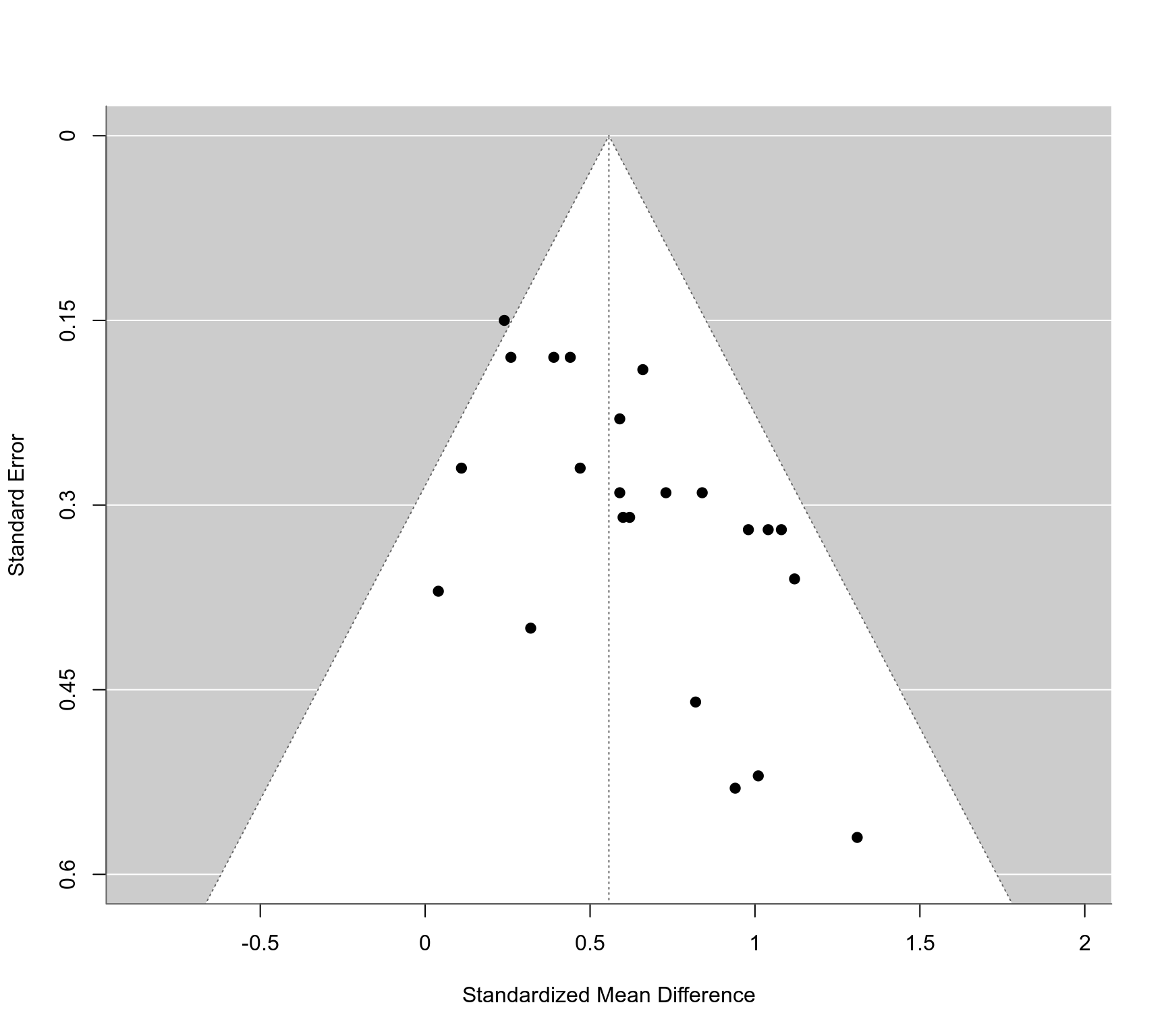 ### rank and regression tests for funnel plot asymmetry
ranktest(res)
#>
#> Rank Correlation Test for Funnel Plot Asymmetry
#>
#> Kendall's tau = 0.4284, p = 0.0049
#>
regtest(res)
#>
#> Regression Test for Funnel Plot Asymmetry
#>
#> Model: mixed-effects meta-regression model
#> Predictor: standard error
#>
#> Test for Funnel Plot Asymmetry: z = 3.1763, p = 0.0015
#> Limit Estimate (as sei -> 0): b = 0.0519 (CI: -0.2615, 0.3653)
#>
### meta-regression analyses examining various potential moderators
rma(smd, sei=se, mods = ~ score, data=dat, method="DL")
#>
#> Mixed-Effects Model (k = 23; tau^2 estimator: DL)
#>
#> tau^2 (estimated amount of residual heterogeneity): 0.0181 (SE = 0.0280)
#> tau (square root of estimated tau^2 value): 0.1347
#> I^2 (residual heterogeneity / unaccounted variability): 20.21%
#> H^2 (unaccounted variability / sampling variability): 1.25
#> R^2 (amount of heterogeneity accounted for): 0.00%
#>
#> Test for Residual Heterogeneity:
#> QE(df = 21) = 26.3177, p-val = 0.1946
#>
#> Test of Moderators (coefficient 2):
#> QM(df = 1) = 1.1320, p-val = 0.2874
#>
#> Model Results:
#>
#> estimate se zval pval ci.lb ci.ub
#> intrcpt 0.8883 0.3176 2.7974 0.0052 0.2659 1.5107 **
#> score -0.0424 0.0398 -1.0639 0.2874 -0.1204 0.0357
#>
#> ---
#> Signif. codes: 0 ‘***’ 0.001 ‘**’ 0.01 ‘*’ 0.05 ‘.’ 0.1 ‘ ’ 1
#>
rma(smd, sei=se, mods = ~ alloconc, data=dat, method="DL")
#>
#> Mixed-Effects Model (k = 23; tau^2 estimator: DL)
#>
#> tau^2 (estimated amount of residual heterogeneity): 0.0227 (SE = 0.0299)
#> tau (square root of estimated tau^2 value): 0.1507
#> I^2 (residual heterogeneity / unaccounted variability): 23.78%
#> H^2 (unaccounted variability / sampling variability): 1.31
#> R^2 (amount of heterogeneity accounted for): 0.00%
#>
#> Test for Residual Heterogeneity:
#> QE(df = 21) = 27.5502, p-val = 0.1534
#>
#> Test of Moderators (coefficient 2):
#> QM(df = 1) = 0.0417, p-val = 0.8383
#>
#> Model Results:
#>
#> estimate se zval pval ci.lb ci.ub
#> intrcpt 0.5786 0.1041 5.5588 <.0001 0.3746 0.7827 ***
#> alloconc -0.0275 0.1348 -0.2041 0.8383 -0.2917 0.2366
#>
#> ---
#> Signif. codes: 0 ‘***’ 0.001 ‘**’ 0.01 ‘*’ 0.05 ‘.’ 0.1 ‘ ’ 1
#>
rma(smd, sei=se, mods = ~ blind, data=dat, method="DL")
#>
#> Mixed-Effects Model (k = 23; tau^2 estimator: DL)
#>
#> tau^2 (estimated amount of residual heterogeneity): 0.0226 (SE = 0.0298)
#> tau (square root of estimated tau^2 value): 0.1502
#> I^2 (residual heterogeneity / unaccounted variability): 23.65%
#> H^2 (unaccounted variability / sampling variability): 1.31
#> R^2 (amount of heterogeneity accounted for): 0.00%
#>
#> Test for Residual Heterogeneity:
#> QE(df = 21) = 27.5032, p-val = 0.1548
#>
#> Test of Moderators (coefficient 2):
#> QM(df = 1) = 0.0695, p-val = 0.7921
#>
#> Model Results:
#>
#> estimate se zval pval ci.lb ci.ub
#> intrcpt 0.5809 0.0972 5.9752 <.0001 0.3903 0.7714 ***
#> blind -0.0349 0.1325 -0.2635 0.7921 -0.2946 0.2248
#>
#> ---
#> Signif. codes: 0 ‘***’ 0.001 ‘**’ 0.01 ‘*’ 0.05 ‘.’ 0.1 ‘ ’ 1
#>
rma(smd, sei=se, mods = ~ itt, data=dat, method="DL")
#>
#> Mixed-Effects Model (k = 23; tau^2 estimator: DL)
#>
#> tau^2 (estimated amount of residual heterogeneity): 0.0224 (SE = 0.0298)
#> tau (square root of estimated tau^2 value): 0.1495
#> I^2 (residual heterogeneity / unaccounted variability): 23.49%
#> H^2 (unaccounted variability / sampling variability): 1.31
#> R^2 (amount of heterogeneity accounted for): 0.00%
#>
#> Test for Residual Heterogeneity:
#> QE(df = 21) = 27.4459, p-val = 0.1566
#>
#> Test of Moderators (coefficient 2):
#> QM(df = 1) = 0.0360, p-val = 0.8496
#>
#> Model Results:
#>
#> estimate se zval pval ci.lb ci.ub
#> intrcpt 0.5496 0.0926 5.9355 <.0001 0.3681 0.7310 ***
#> itt 0.0250 0.1319 0.1897 0.8496 -0.2336 0.2836
#>
#> ---
#> Signif. codes: 0 ‘***’ 0.001 ‘**’ 0.01 ‘*’ 0.05 ‘.’ 0.1 ‘ ’ 1
#>
rma(smd, sei=se, mods = ~ duration, data=dat, method="DL")
#>
#> Mixed-Effects Model (k = 23; tau^2 estimator: DL)
#>
#> tau^2 (estimated amount of residual heterogeneity): 0.0230 (SE = 0.0304)
#> tau (square root of estimated tau^2 value): 0.1516
#> I^2 (residual heterogeneity / unaccounted variability): 23.62%
#> H^2 (unaccounted variability / sampling variability): 1.31
#> R^2 (amount of heterogeneity accounted for): 0.00%
#>
#> Test for Residual Heterogeneity:
#> QE(df = 21) = 27.4927, p-val = 0.1551
#>
#> Test of Moderators (coefficient 2):
#> QM(df = 1) = 0.0004, p-val = 0.9849
#>
#> Model Results:
#>
#> estimate se zval pval ci.lb ci.ub
#> intrcpt 0.5601 0.1451 3.8605 0.0001 0.2757 0.8444 ***
#> duration 0.0002 0.0088 0.0190 0.9849 -0.0171 0.0174
#>
#> ---
#> Signif. codes: 0 ‘***’ 0.001 ‘**’ 0.01 ‘*’ 0.05 ‘.’ 0.1 ‘ ’ 1
#>
rma(smd, sei=se, mods = ~ tailor, data=dat, method="DL")
#>
#> Mixed-Effects Model (k = 23; tau^2 estimator: DL)
#>
#> tau^2 (estimated amount of residual heterogeneity): 0.0074 (SE = 0.0252)
#> tau (square root of estimated tau^2 value): 0.0863
#> I^2 (residual heterogeneity / unaccounted variability): 9.14%
#> H^2 (unaccounted variability / sampling variability): 1.10
#> R^2 (amount of heterogeneity accounted for): 58.32%
#>
#> Test for Residual Heterogeneity:
#> QE(df = 21) = 23.1124, p-val = 0.3380
#>
#> Test of Moderators (coefficient 2):
#> QM(df = 1) = 3.5474, p-val = 0.0596
#>
#> Model Results:
#>
#> estimate se zval pval ci.lb ci.ub
#> intrcpt 0.3717 0.1084 3.4281 0.0006 0.1592 0.5843 ***
#> tailor 0.2434 0.1292 1.8835 0.0596 -0.0099 0.4967 .
#>
#> ---
#> Signif. codes: 0 ‘***’ 0.001 ‘**’ 0.01 ‘*’ 0.05 ‘.’ 0.1 ‘ ’ 1
#>
rma(smd, sei=se, mods = ~ pperf, data=dat, method="DL")
#> Warning: 2 studies with NAs omitted from model fitting.
#>
#> Mixed-Effects Model (k = 21; tau^2 estimator: DL)
#>
#> tau^2 (estimated amount of residual heterogeneity): 0 (SE = 0.0237)
#> tau (square root of estimated tau^2 value): 0
#> I^2 (residual heterogeneity / unaccounted variability): 0.00%
#> H^2 (unaccounted variability / sampling variability): 1.00
#> R^2 (amount of heterogeneity accounted for): 100.00%
#>
#> Test for Residual Heterogeneity:
#> QE(df = 19) = 17.1739, p-val = 0.5781
#>
#> Test of Moderators (coefficient 2):
#> QM(df = 1) = 7.3013, p-val = 0.0069
#>
#> Model Results:
#>
#> estimate se zval pval ci.lb ci.ub
#> intrcpt 0.7318 0.0997 7.3429 <.0001 0.5365 0.9272 ***
#> pperf -0.0137 0.0051 -2.7021 0.0069 -0.0236 -0.0038 **
#>
#> ---
#> Signif. codes: 0 ‘***’ 0.001 ‘**’ 0.01 ‘*’ 0.05 ‘.’ 0.1 ‘ ’ 1
#>
rma(smd, sei=se, mods = ~ I(meetings * hours), data=dat, method="DL")
#>
#> Mixed-Effects Model (k = 23; tau^2 estimator: DL)
#>
#> tau^2 (estimated amount of residual heterogeneity): 0.0075 (SE = 0.0239)
#> tau (square root of estimated tau^2 value): 0.0867
#> I^2 (residual heterogeneity / unaccounted variability): 9.72%
#> H^2 (unaccounted variability / sampling variability): 1.11
#> R^2 (amount of heterogeneity accounted for): 57.90%
#>
#> Test for Residual Heterogeneity:
#> QE(df = 21) = 23.2607, p-val = 0.3302
#>
#> Test of Moderators (coefficient 2):
#> QM(df = 1) = 3.8574, p-val = 0.0495
#>
#> Model Results:
#>
#> estimate se zval pval ci.lb ci.ub
#> intrcpt 0.4453 0.0773 5.7644 <.0001 0.2939 0.5968 ***
#> I(meetings * hours) 0.0073 0.0037 1.9640 0.0495 0.0000 0.0146 *
#>
#> ---
#> Signif. codes: 0 ‘***’ 0.001 ‘**’ 0.01 ‘*’ 0.05 ‘.’ 0.1 ‘ ’ 1
#>
### rank and regression tests for funnel plot asymmetry
ranktest(res)
#>
#> Rank Correlation Test for Funnel Plot Asymmetry
#>
#> Kendall's tau = 0.4284, p = 0.0049
#>
regtest(res)
#>
#> Regression Test for Funnel Plot Asymmetry
#>
#> Model: mixed-effects meta-regression model
#> Predictor: standard error
#>
#> Test for Funnel Plot Asymmetry: z = 3.1763, p = 0.0015
#> Limit Estimate (as sei -> 0): b = 0.0519 (CI: -0.2615, 0.3653)
#>
### meta-regression analyses examining various potential moderators
rma(smd, sei=se, mods = ~ score, data=dat, method="DL")
#>
#> Mixed-Effects Model (k = 23; tau^2 estimator: DL)
#>
#> tau^2 (estimated amount of residual heterogeneity): 0.0181 (SE = 0.0280)
#> tau (square root of estimated tau^2 value): 0.1347
#> I^2 (residual heterogeneity / unaccounted variability): 20.21%
#> H^2 (unaccounted variability / sampling variability): 1.25
#> R^2 (amount of heterogeneity accounted for): 0.00%
#>
#> Test for Residual Heterogeneity:
#> QE(df = 21) = 26.3177, p-val = 0.1946
#>
#> Test of Moderators (coefficient 2):
#> QM(df = 1) = 1.1320, p-val = 0.2874
#>
#> Model Results:
#>
#> estimate se zval pval ci.lb ci.ub
#> intrcpt 0.8883 0.3176 2.7974 0.0052 0.2659 1.5107 **
#> score -0.0424 0.0398 -1.0639 0.2874 -0.1204 0.0357
#>
#> ---
#> Signif. codes: 0 ‘***’ 0.001 ‘**’ 0.01 ‘*’ 0.05 ‘.’ 0.1 ‘ ’ 1
#>
rma(smd, sei=se, mods = ~ alloconc, data=dat, method="DL")
#>
#> Mixed-Effects Model (k = 23; tau^2 estimator: DL)
#>
#> tau^2 (estimated amount of residual heterogeneity): 0.0227 (SE = 0.0299)
#> tau (square root of estimated tau^2 value): 0.1507
#> I^2 (residual heterogeneity / unaccounted variability): 23.78%
#> H^2 (unaccounted variability / sampling variability): 1.31
#> R^2 (amount of heterogeneity accounted for): 0.00%
#>
#> Test for Residual Heterogeneity:
#> QE(df = 21) = 27.5502, p-val = 0.1534
#>
#> Test of Moderators (coefficient 2):
#> QM(df = 1) = 0.0417, p-val = 0.8383
#>
#> Model Results:
#>
#> estimate se zval pval ci.lb ci.ub
#> intrcpt 0.5786 0.1041 5.5588 <.0001 0.3746 0.7827 ***
#> alloconc -0.0275 0.1348 -0.2041 0.8383 -0.2917 0.2366
#>
#> ---
#> Signif. codes: 0 ‘***’ 0.001 ‘**’ 0.01 ‘*’ 0.05 ‘.’ 0.1 ‘ ’ 1
#>
rma(smd, sei=se, mods = ~ blind, data=dat, method="DL")
#>
#> Mixed-Effects Model (k = 23; tau^2 estimator: DL)
#>
#> tau^2 (estimated amount of residual heterogeneity): 0.0226 (SE = 0.0298)
#> tau (square root of estimated tau^2 value): 0.1502
#> I^2 (residual heterogeneity / unaccounted variability): 23.65%
#> H^2 (unaccounted variability / sampling variability): 1.31
#> R^2 (amount of heterogeneity accounted for): 0.00%
#>
#> Test for Residual Heterogeneity:
#> QE(df = 21) = 27.5032, p-val = 0.1548
#>
#> Test of Moderators (coefficient 2):
#> QM(df = 1) = 0.0695, p-val = 0.7921
#>
#> Model Results:
#>
#> estimate se zval pval ci.lb ci.ub
#> intrcpt 0.5809 0.0972 5.9752 <.0001 0.3903 0.7714 ***
#> blind -0.0349 0.1325 -0.2635 0.7921 -0.2946 0.2248
#>
#> ---
#> Signif. codes: 0 ‘***’ 0.001 ‘**’ 0.01 ‘*’ 0.05 ‘.’ 0.1 ‘ ’ 1
#>
rma(smd, sei=se, mods = ~ itt, data=dat, method="DL")
#>
#> Mixed-Effects Model (k = 23; tau^2 estimator: DL)
#>
#> tau^2 (estimated amount of residual heterogeneity): 0.0224 (SE = 0.0298)
#> tau (square root of estimated tau^2 value): 0.1495
#> I^2 (residual heterogeneity / unaccounted variability): 23.49%
#> H^2 (unaccounted variability / sampling variability): 1.31
#> R^2 (amount of heterogeneity accounted for): 0.00%
#>
#> Test for Residual Heterogeneity:
#> QE(df = 21) = 27.4459, p-val = 0.1566
#>
#> Test of Moderators (coefficient 2):
#> QM(df = 1) = 0.0360, p-val = 0.8496
#>
#> Model Results:
#>
#> estimate se zval pval ci.lb ci.ub
#> intrcpt 0.5496 0.0926 5.9355 <.0001 0.3681 0.7310 ***
#> itt 0.0250 0.1319 0.1897 0.8496 -0.2336 0.2836
#>
#> ---
#> Signif. codes: 0 ‘***’ 0.001 ‘**’ 0.01 ‘*’ 0.05 ‘.’ 0.1 ‘ ’ 1
#>
rma(smd, sei=se, mods = ~ duration, data=dat, method="DL")
#>
#> Mixed-Effects Model (k = 23; tau^2 estimator: DL)
#>
#> tau^2 (estimated amount of residual heterogeneity): 0.0230 (SE = 0.0304)
#> tau (square root of estimated tau^2 value): 0.1516
#> I^2 (residual heterogeneity / unaccounted variability): 23.62%
#> H^2 (unaccounted variability / sampling variability): 1.31
#> R^2 (amount of heterogeneity accounted for): 0.00%
#>
#> Test for Residual Heterogeneity:
#> QE(df = 21) = 27.4927, p-val = 0.1551
#>
#> Test of Moderators (coefficient 2):
#> QM(df = 1) = 0.0004, p-val = 0.9849
#>
#> Model Results:
#>
#> estimate se zval pval ci.lb ci.ub
#> intrcpt 0.5601 0.1451 3.8605 0.0001 0.2757 0.8444 ***
#> duration 0.0002 0.0088 0.0190 0.9849 -0.0171 0.0174
#>
#> ---
#> Signif. codes: 0 ‘***’ 0.001 ‘**’ 0.01 ‘*’ 0.05 ‘.’ 0.1 ‘ ’ 1
#>
rma(smd, sei=se, mods = ~ tailor, data=dat, method="DL")
#>
#> Mixed-Effects Model (k = 23; tau^2 estimator: DL)
#>
#> tau^2 (estimated amount of residual heterogeneity): 0.0074 (SE = 0.0252)
#> tau (square root of estimated tau^2 value): 0.0863
#> I^2 (residual heterogeneity / unaccounted variability): 9.14%
#> H^2 (unaccounted variability / sampling variability): 1.10
#> R^2 (amount of heterogeneity accounted for): 58.32%
#>
#> Test for Residual Heterogeneity:
#> QE(df = 21) = 23.1124, p-val = 0.3380
#>
#> Test of Moderators (coefficient 2):
#> QM(df = 1) = 3.5474, p-val = 0.0596
#>
#> Model Results:
#>
#> estimate se zval pval ci.lb ci.ub
#> intrcpt 0.3717 0.1084 3.4281 0.0006 0.1592 0.5843 ***
#> tailor 0.2434 0.1292 1.8835 0.0596 -0.0099 0.4967 .
#>
#> ---
#> Signif. codes: 0 ‘***’ 0.001 ‘**’ 0.01 ‘*’ 0.05 ‘.’ 0.1 ‘ ’ 1
#>
rma(smd, sei=se, mods = ~ pperf, data=dat, method="DL")
#> Warning: 2 studies with NAs omitted from model fitting.
#>
#> Mixed-Effects Model (k = 21; tau^2 estimator: DL)
#>
#> tau^2 (estimated amount of residual heterogeneity): 0 (SE = 0.0237)
#> tau (square root of estimated tau^2 value): 0
#> I^2 (residual heterogeneity / unaccounted variability): 0.00%
#> H^2 (unaccounted variability / sampling variability): 1.00
#> R^2 (amount of heterogeneity accounted for): 100.00%
#>
#> Test for Residual Heterogeneity:
#> QE(df = 19) = 17.1739, p-val = 0.5781
#>
#> Test of Moderators (coefficient 2):
#> QM(df = 1) = 7.3013, p-val = 0.0069
#>
#> Model Results:
#>
#> estimate se zval pval ci.lb ci.ub
#> intrcpt 0.7318 0.0997 7.3429 <.0001 0.5365 0.9272 ***
#> pperf -0.0137 0.0051 -2.7021 0.0069 -0.0236 -0.0038 **
#>
#> ---
#> Signif. codes: 0 ‘***’ 0.001 ‘**’ 0.01 ‘*’ 0.05 ‘.’ 0.1 ‘ ’ 1
#>
rma(smd, sei=se, mods = ~ I(meetings * hours), data=dat, method="DL")
#>
#> Mixed-Effects Model (k = 23; tau^2 estimator: DL)
#>
#> tau^2 (estimated amount of residual heterogeneity): 0.0075 (SE = 0.0239)
#> tau (square root of estimated tau^2 value): 0.0867
#> I^2 (residual heterogeneity / unaccounted variability): 9.72%
#> H^2 (unaccounted variability / sampling variability): 1.11
#> R^2 (amount of heterogeneity accounted for): 57.90%
#>
#> Test for Residual Heterogeneity:
#> QE(df = 21) = 23.2607, p-val = 0.3302
#>
#> Test of Moderators (coefficient 2):
#> QM(df = 1) = 3.8574, p-val = 0.0495
#>
#> Model Results:
#>
#> estimate se zval pval ci.lb ci.ub
#> intrcpt 0.4453 0.0773 5.7644 <.0001 0.2939 0.5968 ***
#> I(meetings * hours) 0.0073 0.0037 1.9640 0.0495 0.0000 0.0146 *
#>
#> ---
#> Signif. codes: 0 ‘***’ 0.001 ‘**’ 0.01 ‘*’ 0.05 ‘.’ 0.1 ‘ ’ 1
#>