Variance Inflation Factors for 'rma' Objects

Function to compute (generalized) variance inflation factors (VIFs) for objects of class "rma".

vif(x, ...)

# S3 method for class 'rma'
vif(x, btt, att, table=FALSE, reestimate=FALSE, sim=FALSE, progbar=TRUE,
    seed=NULL, parallel="no", ncpus=1, cl, digits, ...)

# S3 method for class 'vif.rma'
print(x, digits=x$digits, ...)

Arguments

x

an object of class "rma" (for vif) or "vif.rma" (for print).

btt

optional vector of indices (or list thereof) to specify a set of coefficients for which a generalized variance inflation factor (GVIF) should be computed. Can also be a string to grep for.

att

optional vector of indices (or list thereof) to specify a set of scale coefficients for which a generalized variance inflation factor (GVIF) should be computed. Can also be a string to grep for. Only relevant for location-scale models (see rma.uni).

table

logical to specify whether the VIFs should be added to the model coefficient table (the default is FALSE). Only relevant when btt (or att) is not specified.

reestimate

logical to specify whether the model should be reestimated when removing moderator variables from the model for computing a (G)VIF (the default is FALSE).

sim

logical to specify whether the distribution of each (G)VIF under independence should be simulated (the default is FALSE). Can also be an integer to specify how many values to simulate (when sim=TRUE, the default is 1000).

progbar

logical to specify whether a progress bar should be shown when sim=TRUE (the default is TRUE).

seed

optional value to specify the seed of the random number generator when sim=TRUE (for reproducibility).

parallel

character string to specify whether parallel processing should be used (the default is "no"). For parallel processing, set to either "snow" or "multicore". See ‘Note’.

ncpus

integer to specify the number of processes to use in the parallel processing.

cl

optional cluster to use if parallel="snow". If unspecified, a cluster on the local machine is created for the duration of the call.

digits

optional integer to specify the number of decimal places to which the printed results should be rounded. If unspecified, the default is to take the value from the object.

...

other arguments.

Details

The function computes (generalized) variance inflation factors (VIFs) for meta-regression models. Hence, the model specified via argument x must include moderator variables (and more than one for this to be useful, as the VIF for a model with a single moderator variable will always be equal to 1).

VIFs for Individual Coefficients

By default (i.e., if btt is not specified), VIFs are computed for the individual model coefficients.

Let \(b_j\) denote the estimate of the \(j\text{th}\) model coefficient of a particular meta-regression model and \(\text{Var}[b_j]\) its variance (i.e., the corresponding diagonal element from the matrix obtained with the vcov function). Moreover, let \(b'_j\) denote the estimate of the same model coefficient if the other moderator variables in the model had not been included in the model and \(\text{Var}[b'_j]\) the corresponding variance. Then the VIF for the model coefficient is given by \[\text{VIF}[b_j] = \frac{\text{Var}[b_j]}{\text{Var}[b'_j]},\] which indicates the inflation in the variance of the estimated model coefficient due to potential collinearity of the \(j\text{th}\) moderator variable with the other moderator variables in the model. Taking the square root of a VIF gives the corresponding standard error inflation factor (SIF).

GVIFs for Sets of Coefficients

If the model includes factors (coded in terms of multiple dummy variables) or other sets of moderator variables that belong together (e.g., for polynomials or cubic splines), one may want to examine how much the variance in all of the coefficients in the set is jointly impacted by collinearity with the other moderator variables in the model. For this, we can compute a generalized variance inflation factor (GVIF) (Fox & Monette, 1992) by setting the btt argument equal to the indices of those coefficients for which the GVIF should be computed. The square root of a GVIF indicates the inflation in the confidence ellipse/(hyper)ellipsoid for the set of coefficients corresponding to the set due to collinearity. However, to make this value more directly comparable to SIFs (based on single coefficients), the function computes the generalized standard error inflation factor (GSIF) by raising the GVIF to the power of \(1/(2m)\) (where \(m\) denotes the number of coefficients in the set). One can also specify a list of indices/strings, in which case GVIFs/GSIFs of all list elements will be computed. See ‘Examples’.

For location-scale models fitted with the rma.uni function, one can use the att argument in an analogous manner to specify the indices of the scale coefficients for which a GVIF should be computed.

Re-Estimating the Model

The way the VIF is typically computed for a particular model coefficient (or a set thereof for a GVIF) makes use of some clever linear algebra to avoid having to re-estimate the model when removing the other moderator variables from the model. This speeds up the computations considerably. However, this assumes that the other moderator variables do not impact other aspects of the model, in particular the amount of residual heterogeneity (or, more generally, any variance/correlation components in a more complex model, such as those that can be fitted with the rma.mv function).

For a more accurate (but slower) computation of each (G)VIF, one can set reestimate=TRUE, in which case the model is refitted to account for the impact that removal of the other moderator variables has on all aspects of the model. Note that refitting may fail, in which case the corresponding (G)VIF will be missing.

Interpreting the Size of (G)VIFs

A large VIF value suggests that the precision with which we can estimate a particular model coefficient (or a set thereof for a GVIF) is negatively impacted by multicollinearity among the moderator variables. However, there is no specific cutoff for determining whether a particular (G)VIF is ‘large’. Sometimes, values such as 5 or 10 have been suggested as rules of thumb, but such cutoffs are essentially arbitrary.

Simulating the Distribution of (G)VIFs Under Independence

As a more principled approach, we can simulate the distribution of a particular (G)VIF under independence and then examine how extreme the actually observed (G)VIF value is under this distribution. The distribution is simulated by randomly reshuffling the columns of the model matrix (to break any dependence between the moderators) and recomputing the (G)VIF. When setting sim=TRUE, this is done 1000 times (but one can also set sim to an integer to specify how many (G)VIF values should be simulated).

The way the model matrix is reshuffled depends on how the model was fitted. When the model was specified as a formula via the mods argument and the data was supplied via the data argument, then each column of the data frame specified via data is reshuffled and the formula is evaluated within the reshuffled data (creating the corresponding reshuffled model matrix). This way, factor/character variables are properly reshuffled and derived terms (e.g., interactions, polynomials, splines) are correct constructed. This is the recommended approach.

On the other hand, if the model matrix was directly supplied to the mods argument, then each column of the matrix is directly reshuffled. This is not recommended, since this approach cannot account for any inherent relationships between variables in the model matrix (e.g., an interaction term is the product of two variables and should not be reshuffled by itself).

Once the distribution of a (G)VIF under independence has been simulated, the proportion of simulated values that are smaller than the actually observed (G)VIF value is computed. If the proportion is close to 1, then this indicates that the actually observed (G)VIF value is extreme.

The general principle underlying the simulation approach is the same as that underlying Horn's parallel analysis (1965) for determining the number of components / factors to keep in a principal component / factor analysis.

Value

An object of class "vif.rma". The object is a list containing the following components:

vif

a list of data frames with the (G)VIFs and (G)SIFs and some additional information.

vifs

a vector with the (G)VIFs.

table

the model coefficient table (only when table=TRUE).

sim

a matrix with the simulated (G)VIF values (only when sim=TRUE).

prop

a vector with the proportions of simulated values that are smaller than the actually observed (G)VIF values (only when sim=TRUE).

...

some additional elements/values.

When x was a location-scale model object and (G)VIFs can be computed for both the location and the scale coefficients, then the object is a list with elements beta and alpha, where each element is a "vif.rma" object as described above.

The results are formatted and printed with the print function. To format the results as a data frame, one can use the as.data.frame function. When sim=TRUE, the distribution of each (G)VIF can be plotted with the plot function.

Note

If the original model fitted involved redundant predictors that were dropped from the model, then sim=TRUE cannot be used. In this case, one should remove any redundancies in the original model fitted before using this method.

When using sim=TRUE, the model needs to be refitted (by default) 1000 times. When sim=TRUE is combined with reestimate=TRUE, then this value needs to be multiplied by the total number of (G)VIF values that are computed by the function. Hence, the combination of sim=TRUE with reestimate=TRUE is computationally expensive, especially for more complex models where model fitting can be slow.

When refitting the model fails, the simulated (G)VIF value(s) will be missing. It can also happen that one or multiple model coefficients become inestimable due to redundancies in the model matrix after the reshuffling. In this case, the corresponding simulated (G)VIF value(s) will be set to Inf (as that is the value of (G)VIFs in the limit as we approach perfect multicollinearity).

On machines with multiple cores, one can try to speed things up by delegating the model fitting to separate worker processes, that is, by setting parallel="snow" or parallel="multicore" and ncpus to some value larger than 1. Parallel processing makes use of the parallel package, using the makePSOCKcluster and parLapply functions when parallel="snow" or using mclapply when parallel="multicore" (the latter only works on Unix/Linux-alikes). With parallel::detectCores(), one can check on the number of available cores on the local machine.

Author

Wolfgang Viechtbauer (wvb@metafor-project.org, https://www.metafor-project.org).

References

Belsley, D. A., Kuh, E., & Welsch, R. E. (1980). Regression diagnostics. New York: Wiley.

Fox, J., & Monette, G. (1992). Generalized collinearity diagnostics. Journal of the American Statistical Association, 87(417), 178–183. https://doi.org/10.2307/2290467

Horn, J. L. (1965). A rationale and test for the number of factors in factor analysis. Psychometrika, 30(2), 179–185. https://doi.org/10.1007/BF02289447

Stewart, G. W. (1987). Collinearity and least squares regression. Statistical Science, 2(1), 68–84. https://doi.org/10.1214/ss/1177013439

Wax, Y. (1992). Collinearity diagnosis for a relative risk regression-analysis: An application to assessment of diet cancer relationship in epidemiologic studies. Statistics in Medicine, 11(10), 1273–1287. https://doi.org/10.1002/sim.4780111003

Viechtbauer, W. (2010). Conducting meta-analyses in R with the metafor package. Journal of Statistical Software, 36(3), 1–48. https://doi.org/10.18637/jss.v036.i03

Viechtbauer, W., & López-López, J. A. (2022). Location-scale models for meta-analysis. Research Synthesis Methods. 13(6), 697–715. https://doi.org/10.1002/jrsm.1562

See also

rma.uni, rma.glmm, and rma.mv for functions to fit models for which variance inflation factors can be computed.

plot for the plot method and as.data.frame for the method to format the results as a data frame.

Examples

### copy data from Bangert-Drowns et al. (2004) into 'dat'
dat <- dat.bangertdrowns2004

### fit mixed-effects meta-regression model
res <- rma(yi, vi, mods = ~ length + wic + feedback + info + pers + imag + meta, data=dat)
#> Warning: 7 studies with NAs omitted from model fitting.

### get variance inflation factors
vif(res)
#> 
#> length     wic  feedback    info    pers    imag    meta 
#> 1.5371  1.3860    1.6490  1.8340  5.6780  1.1554  4.5333 
#> 

### use the simulation approach to analyze the size of the VIFs
vif(res, sim=TRUE, seed=1234)
#> 
#>              vif  prop 
#> length    1.5371  0.95 
#> wic       1.3860  0.86 
#> feedback  1.6490  0.98 
#> info      1.8340  0.98 
#> pers      5.6780  1.00 
#> imag      1.1554  0.47 
#> meta      4.5333  1.00 
#> 

### get variance inflation factors using the re-estimation approach
vif(res, reestimate=TRUE)
#> 
#> length     wic  feedback    info    pers    imag    meta 
#> 1.3877  1.2043    1.5060  1.4980  5.2195  1.4386  4.3244 
#> 

### show that VIFs are not influenced by scaling of the predictors
u <- scale # to standardize the predictors
res <- rma(yi, vi, mods = ~ u(length) + u(wic) + u(feedback) + u(info) +
                            u(pers) + u(imag) + u(meta), data=dat)
#> Warning: 7 studies with NAs omitted from model fitting.
vif(res, reestimate=TRUE)
#> 
#> u(length)  u(wic)  u(feedback)  u(info)  u(pers)  u(imag)  u(meta) 
#>    1.3877  1.2043       1.5060   1.4980   5.2195   1.4386   4.3244 
#> 

### get full table
vif(res, reestimate=TRUE, table=TRUE)
#> 
#>             estimate     se    zval   pval   ci.lb  ci.ub    vif    sif 
#> intrcpt       0.1825 0.0406  4.4898 <.0001  0.1028 0.2621     NA     NA 
#> u(length)     0.0458 0.0496  0.9240 0.3555 -0.0514 0.1431 1.3877 1.1780 
#> u(wic)       -0.0210 0.0487 -0.4308 0.6666 -0.1164 0.0744 1.2043 1.0974 
#> u(feedback)   0.0329 0.0524  0.6265 0.5310 -0.0699 0.1357 1.5060 1.2272 
#> u(info)      -0.0460 0.0418 -1.1006 0.2711 -0.1280 0.0360 1.4980 1.2239 
#> u(pers)      -0.0573 0.0956 -0.5992 0.5490 -0.2446 0.1301 5.2195 2.2846 
#> u(imag)       0.1004 0.0452  2.2233 0.0262  0.0119 0.1890 1.4386 1.1994 
#> u(meta)       0.0981 0.0850  1.1537 0.2486 -0.0685 0.2647 4.3244 2.0795 
#> 

############################################################################

### an example where the VIFs are close to 1, but actually reflect considerable
### multicollinearity as can be seen based on the simulation approach
dat <- dat.mcdaniel1994
dat <- escalc(measure="ZCOR", ri=ri, ni=ni, data=dat)
res <- rma(yi, vi, mods = ~ factor(type) + factor(struct), data=dat)
#> Warning: 15 studies with NAs omitted from model fitting.
res
#> 
#> Mixed-Effects Model (k = 145; tau^2 estimator: REML)
#> 
#> tau^2 (estimated amount of residual heterogeneity):     0.0302 (SE = 0.0054)
#> tau (square root of estimated tau^2 value):             0.1737
#> I^2 (residual heterogeneity / unaccounted variability): 80.11%
#> H^2 (unaccounted variability / sampling variability):   5.03
#> R^2 (amount of heterogeneity accounted for):            0.82%
#> 
#> Test for Residual Heterogeneity:
#> QE(df = 141) = 699.1018, p-val < .0001
#> 
#> Test of Moderators (coefficients 2:4):
#> QM(df = 3) = 4.8181, p-val = 0.1856
#> 
#> Model Results:
#> 
#>                  estimate      se     zval    pval    ci.lb   ci.ub      
#> intrcpt            0.2652  0.0228  11.6339  <.0001   0.2206  0.3099  *** 
#> factor(type)p     -0.0688  0.0916  -0.7506  0.4529  -0.2483  0.1108      
#> factor(type)s      0.0402  0.0622   0.6455  0.5186  -0.0818  0.1622      
#> factor(struct)u   -0.0653  0.0424  -1.5394  0.1237  -0.1485  0.0179      
#> 
#> ---
#> Signif. codes:  0 ‘***’ 0.001 ‘**’ 0.01 ‘*’ 0.05 ‘.’ 0.1 ‘ ’ 1
#> 
vif(res)
#> 
#> factor(type)p  factor(type)s  factor(struct)u 
#>        1.0703         1.0431           1.1107 
#> 

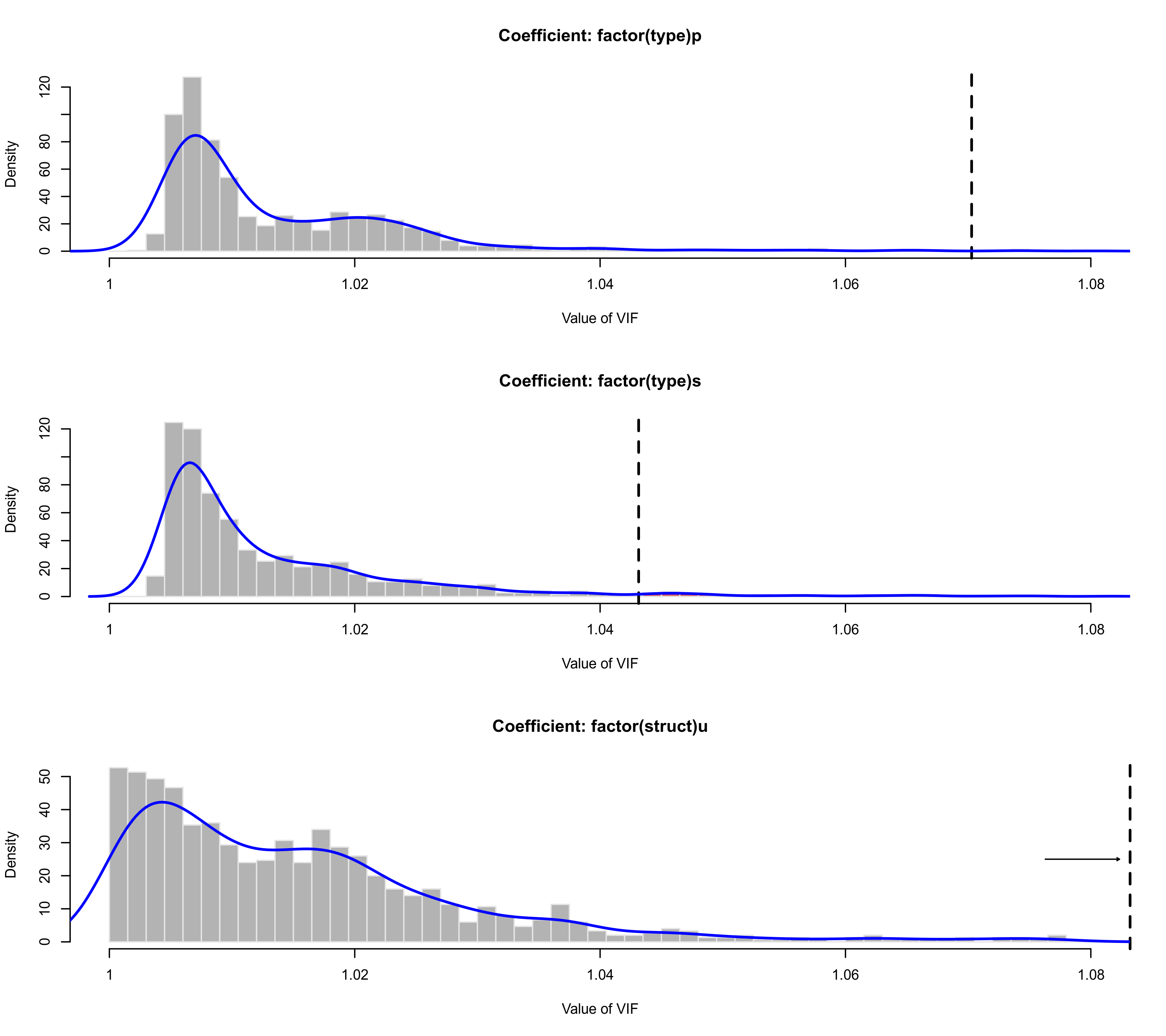
### use the simulation approach to analyze the size of the VIFs
vifs <- vif(res, sim=TRUE, seed=1234)
vifs
#> 
#>                     vif  prop 
#> factor(type)p    1.0703  0.99 
#> factor(type)s    1.0431  0.97 
#> factor(struct)u  1.1107  1.00 
#> 
plot(vifs, lwd=c(2,2), breaks=seq(1,2,by=0.0015), xlim=c(1,1.08))


### an example for a location-scale model
res <- rma(yi, vi, mods = ~ factor(type) + factor(struct),
                   scale = ~ factor(type) + factor(struct), data=dat)
#> Warning: 15 studies with NAs omitted from model fitting.
res
#> 
#> Location-Scale Model (k = 145; tau^2 estimator: REML)
#> 
#> Test for Residual Heterogeneity:
#> QE(df = 141) = 699.1018, p-val < .0001
#> 
#> Test of Location Coefficients (coefficients 2:4):
#> QM(df = 3) = 8.7224, p-val = 0.0332
#> 
#> Model Results (Location):
#> 
#>                  estimate      se     zval    pval    ci.lb   ci.ub      
#> intrcpt            0.2646  0.0260  10.1919  <.0001   0.2137  0.3154  *** 
#> factor(type)p     -0.0707  0.0543  -1.3029  0.1926  -0.1770  0.0356      
#> factor(type)s      0.0287  0.0499   0.5756  0.5649  -0.0691  0.1266      
#> factor(struct)u   -0.0656  0.0357  -1.8385  0.0660  -0.1356  0.0043    . 
#> 
#> Test of Scale Coefficients (coefficients 2:4):
#> QM(df = 3) = 10.0588, p-val = 0.0181
#> 
#> Model Results (Scale):
#> 
#>                  estimate      se      zval    pval     ci.lb    ci.ub      
#> intrcpt           -3.1082  0.2150  -14.4600  <.0001   -3.5295  -2.6869  *** 
#> factor(type)p     -3.1571  9.5670   -0.3300  0.7414  -21.9081  15.5940      
#> factor(type)s     -1.6582  1.0660   -1.5556  0.1198   -3.7474   0.4311      
#> factor(struct)u   -1.4484  0.5121   -2.8285  0.0047   -2.4520  -0.4447   ** 
#> 
#> ---
#> Signif. codes:  0 ‘***’ 0.001 ‘**’ 0.01 ‘*’ 0.05 ‘.’ 0.1 ‘ ’ 1
#> 
vif(res)
#> 
#> Location Coefficients:
#> 
#> factor(type)p  factor(type)s  factor(struct)u 
#>        1.0585         1.1737           1.2137 
#> 
#> Scale Coefficients:
#> 
#> factor(type)p  factor(type)s  factor(struct)u 
#>        1.0069         1.0073           1.0142 
#> 

############################################################################

### calculate log risk ratios and corresponding sampling variances
dat <- escalc(measure="RR", ai=tpos, bi=tneg, ci=cpos, di=cneg, data=dat.bcg)

### fit meta-regression model where one predictor (alloc) is a three-level factor
res <- rma(yi, vi, mods = ~ ablat + alloc + year, data=dat)

### get variance inflation factors for all individual coefficients
vif(res, table=TRUE)
#> 
#>                 estimate      se    zval   pval    ci.lb   ci.ub    vif    sif 
#> intrcpt         -14.4984 38.3943 -0.3776 0.7057 -89.7498 60.7531     NA     NA 
#> ablat            -0.0236  0.0132 -1.7816 0.0748  -0.0495  0.0024 1.7697 1.3303 
#> allocrandom      -0.3421  0.4180 -0.8183 0.4132  -1.1613  0.4772 2.0858 1.4442 
#> allocsystematic   0.0101  0.4467  0.0226 0.9820  -0.8654  0.8856 2.0193 1.4210 
#> year              0.0075  0.0194  0.3849 0.7003  -0.0306  0.0456 1.9148 1.3838 
#> 

### generalized variance inflation factor for the 'alloc' factor
vif(res, btt=3:4)
#> 
#> Collinearity Diagnostics (coefficients 3:4):
#> GVIF = 1.2339, GSIF = 1.0540
#> 

### can also specify a string to grep for
vif(res, btt="alloc")
#> 
#> Collinearity Diagnostics (coefficients 3:4):
#> GVIF = 1.2339, GSIF = 1.0540
#> 

### can also specify a list for the 'btt' argument (and use the simulation approach)
vif(res, btt=list(2,3:4,5), sim=TRUE, seed=1234)
#> 
#>   coefs m    vif    sif prop 
#> 1     2 1 1.7697 1.3303 0.83 
#> 2   3:4 2 1.2339 1.0540 0.23 
#> 3     5 1 1.9148 1.3838 0.87 
#>