Radial (Galbraith) Plots for 'rma' Objects

Function to create radial (also called Galbraith) plots for objects of class "rma".

radial(x, ...)
galbraith(x, ...)

# S3 method for class 'rma'
radial(x, center=FALSE, xlim, zlim, xlab, zlab,
       atz, aty, steps=7, level=x$level, digits=2,
       transf, targs, pch=21, col, bg, back, arc.res=100,
       cex, cex.lab, cex.axis, ...)

Arguments

x: an object of class "rma".
center: logical to specify whether the plot should be centered horizontally at the model estimate (the default is FALSE).
xlim: x-axis limits. If unspecified, the function sets the x-axis limits to some sensible values.
zlim: z-axis limits. If unspecified, the function sets the z-axis limits to some sensible values (note that the z-axis limits are the actual vertical limit of the plotting region).
xlab: title for the x-axis. If unspecified, the function sets an appropriate axis title.
zlab: title for the z-axis. If unspecified, the function sets an appropriate axis title.
atz: position for the z-axis tick marks and labels. If unspecified, these values are set by the function.
aty: position for the y-axis tick marks and labels. If unspecified, these values are set by the function.
steps: the number of tick marks for the y-axis (the default is 7). Ignored when argument aty is used.
level: numeric value between 0 and 100 to specify the level of the z-axis error region. The default is to take the value from the object.
digits: integer to specify the number of decimal places to which the tick mark labels of the y-axis should be rounded (the default is 2).
transf: argument to specify a function to transform the y-axis labels (e.g., transf=exp; see also transf). If unspecified, no transformation is used.
targs: optional arguments needed by the function specified via transf.
pch: plotting symbol. By default, an open circle is used. See points for other options.
col: character string to specify the (border) color of the points.
bg: character string to specify the background color of open plot symbols.
back: character string to specify the background color of the z-axis error region. If unspecified, a shade of gray is used. Set to NA to suppress shading of the region.
arc.res: integer to specify the number of line segments (i.e., the resolution) when drawing the y-axis and confidence interval arcs (the default is 100).
cex: symbol expansion factor.
cex.lab: character expansion factor for axis labels.
cex.axis: character expansion factor for axis annotations.
...: other arguments.

Details

For an equal-effects model, the plot shows the inverse of the standard errors on the horizontal axis (i.e., \(1/\sqrt{v_i}\), where \(v_i\) is the sampling variance of the observed effect size or outcome) against the observed effect sizes or outcomes standardized by their corresponding standard errors on the vertical axis (i.e., \(y_i/\sqrt{v_i}\)). Since the vertical axis corresponds to standardized values, it is referred to as the z-axis within this function. On the right hand side of the plot, an arc is drawn (referred to as the y-axis within this function) corresponding to the observed effect sizes or outcomes. A line projected from (0,0) through a particular point within the plot onto this arc indicates the value of the observed effect size or outcome for that point.

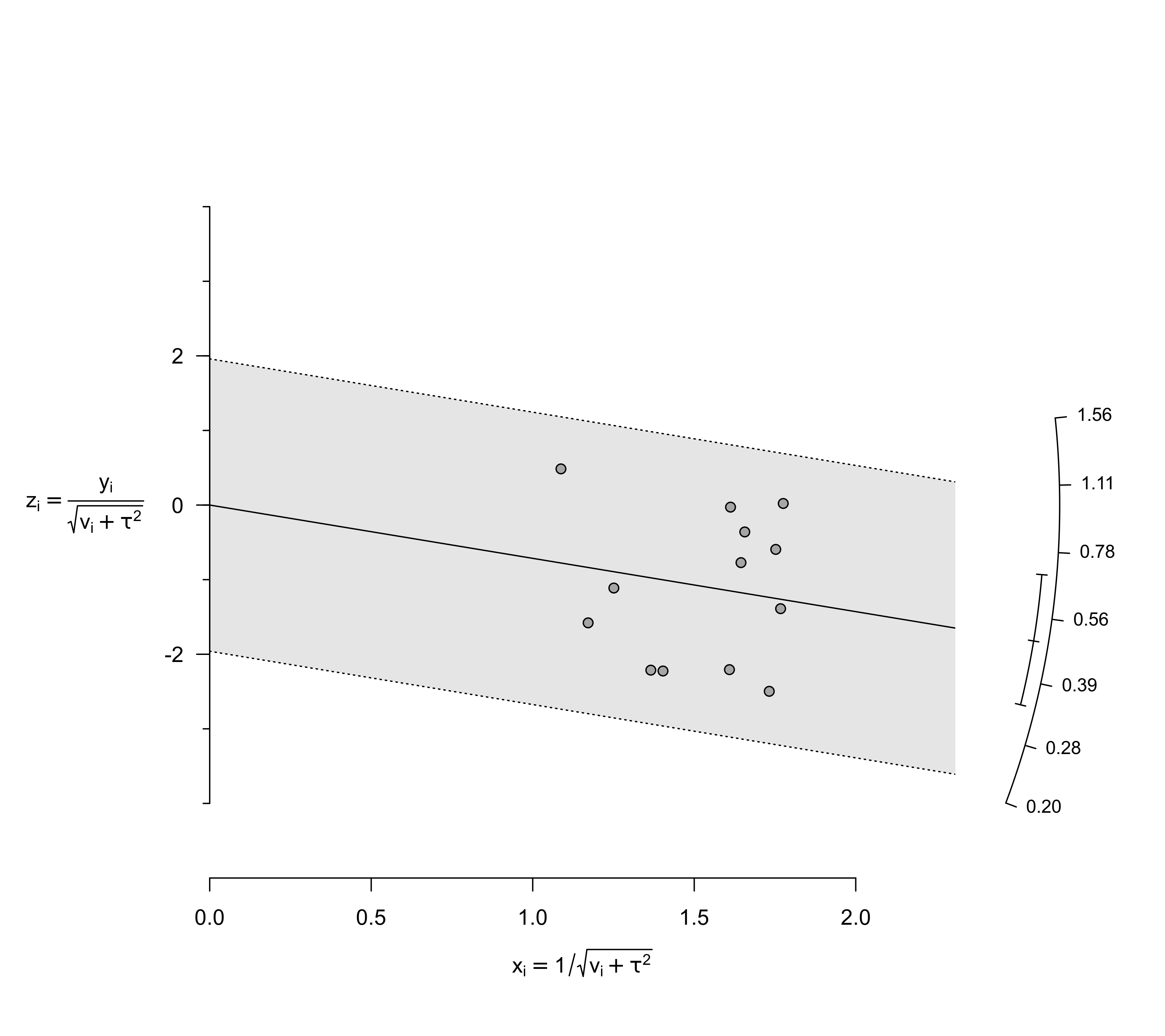
For a random-effects model, the function uses \(1/\sqrt{v_i + \tau^2}\) for the horizontal axis, where \(\tau^2\) is the amount of heterogeneity as estimated based on the model. For the z-axis, \(y_i/\sqrt{v_i + \tau^2}\) is used to compute standardized values of the observed effect sizes or outcomes.

The second (inner/smaller) arc that is drawn on the right hand side indicates the model estimate (in the middle of the arc) and the corresponding confidence interval (at the ends of the arc).

The shaded region in the plot is the z-axis error region. For level=95 (or if this was the level value when the model was fitted), this corresponds to z-axis values equal to \(\pm 1.96\). Under the assumptions of the equal/random-effects models, approximately 95% of the points should fall within this region.

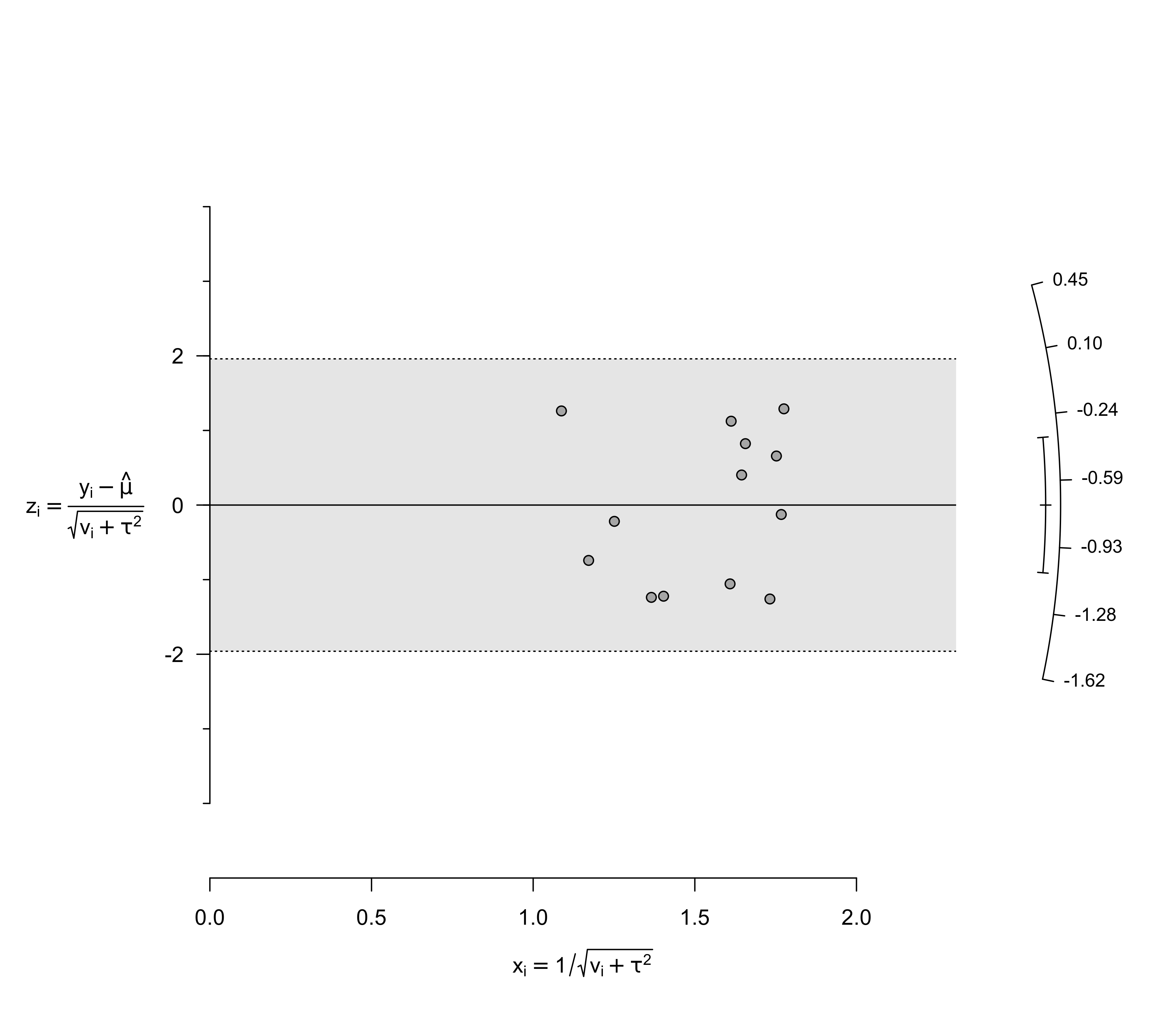
When center=TRUE, the values on the y-axis are centered around the model estimate. As a result, the plot is centered horizontally at the model estimate.

If the z-axis label on the left is too close to the actual z-axis and/or the arc on the right is clipped, then this can be solved by increasing the margins on the right and/or left (see par and in particular the mar argument).

Note that radial plots cannot be drawn for models that contain moderators.

Value

A data frame with components:

x: the x-axis coordinates of the points that were plotted.
y: the y-axis coordinates of the points that were plotted.
ids: the study id numbers.
slab: the study labels.

Note that the data frame is returned invisibly.

Author

Wolfgang Viechtbauer (wvb@metafor-project.org, https://www.metafor-project.org).

References

Galbraith, R. F. (1988). Graphical display of estimates having differing standard errors. Technometrics, 30(3), 271–281. https://doi.org/10.1080/00401706.1988.10488400

Galbraith, R. F. (1988). A note on graphical presentation of estimated odds ratios from several clinical trials. Statistics in Medicine, 7(8), 889–894. https://doi.org/10.1002/sim.4780070807

Galbraith, R. F (1994). Some applications of radial plots. Journal of the American Statistical Association, 89(428), 1232–1242. https://doi.org/10.1080/01621459.1994.10476864

Viechtbauer, W. (2010). Conducting meta-analyses in R with the metafor package. Journal of Statistical Software, 36(3), 1–48. https://doi.org/10.18637/jss.v036.i03

Examples

### calculate log risk ratios and corresponding sampling variances
dat <- escalc(measure="RR", ai=tpos, bi=tneg, ci=cpos, di=cneg, data=dat.bcg)
dat
#> 
#>    trial               author year tpos  tneg cpos  cneg ablat      alloc      yi     vi 
#> 1      1              Aronson 1948    4   119   11   128    44     random -0.8893 0.3256 
#> 2      2     Ferguson & Simes 1949    6   300   29   274    55     random -1.5854 0.1946 
#> 3      3      Rosenthal et al 1960    3   228   11   209    42     random -1.3481 0.4154 
#> 4      4    Hart & Sutherland 1977   62 13536  248 12619    52     random -1.4416 0.0200 
#> 5      5 Frimodt-Moller et al 1973   33  5036   47  5761    13  alternate -0.2175 0.0512 
#> 6      6      Stein & Aronson 1953  180  1361  372  1079    44  alternate -0.7861 0.0069 
#> 7      7     Vandiviere et al 1973    8  2537   10   619    19     random -1.6209 0.2230 
#> 8      8           TPT Madras 1980  505 87886  499 87892    13     random  0.0120 0.0040 
#> 9      9     Coetzee & Berjak 1968   29  7470   45  7232    27     random -0.4694 0.0564 
#> 10    10      Rosenthal et al 1961   17  1699   65  1600    42 systematic -1.3713 0.0730 
#> 11    11       Comstock et al 1974  186 50448  141 27197    18 systematic -0.3394 0.0124 
#> 12    12   Comstock & Webster 1969    5  2493    3  2338    33 systematic  0.4459 0.5325 
#> 13    13       Comstock et al 1976   27 16886   29 17825    33 systematic -0.0173 0.0714 
#> 

### fit equal-effects model
res <- rma(yi, vi, data=dat, method="EE")

### draw radial plot
radial(res)

### the line from (0,0) with a slope equal to the log risk ratio from the 4th study points
### to the corresponding effect size value on the arc (i.e., -1.44)
abline(a=0, b=dat$yi[4], lty="dotted")

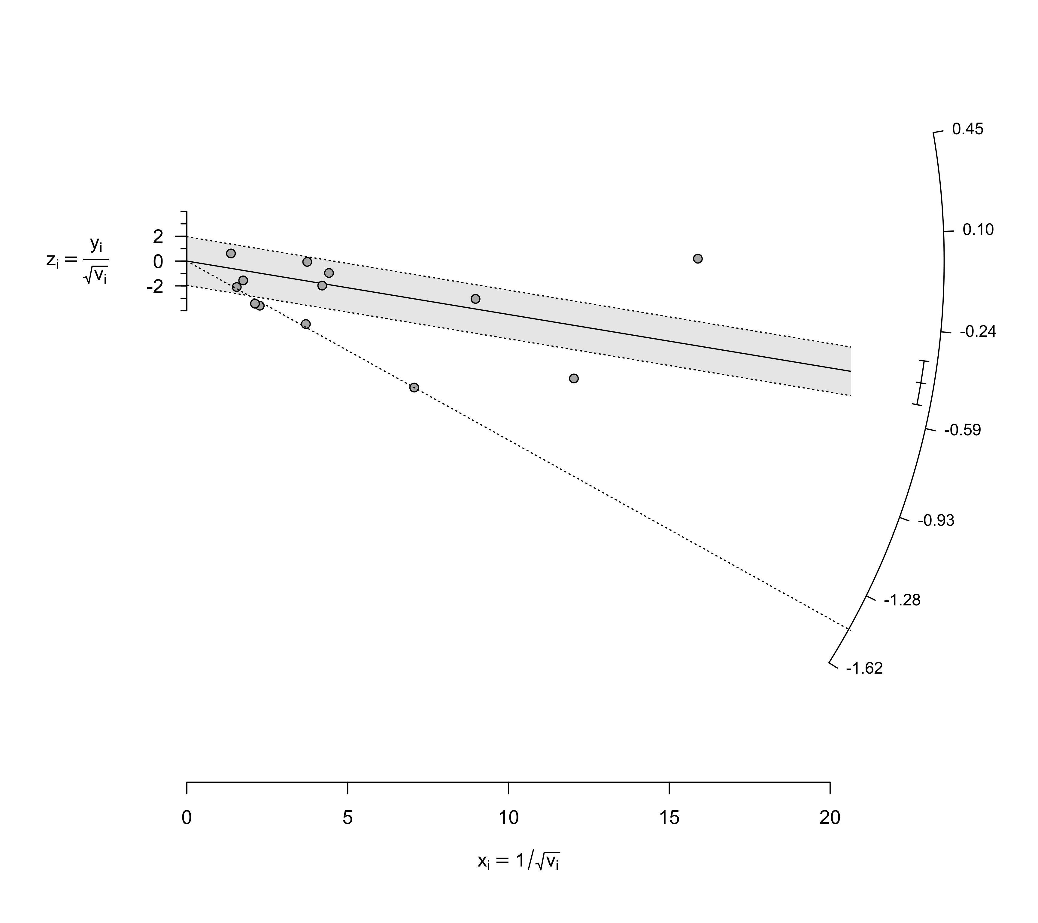dat$yi[4]
#> [1] -1.441551

### meta-analysis of the log risk ratios using a random-effects model
res <- rma(yi, vi, data=dat)

### draw radial plot
radial(res)


### center the values around the model estimate
radial(res, center=TRUE)


### show risk ratio values on the y-axis arc
radial(res, transf=exp)