Plot Method for 'infl.rma.uni' Objects
plot.infl.rma.uni.RdFunction to plot objects of class "infl.rma.uni".
# S3 method for class 'infl.rma.uni'
plot(x, plotinf=TRUE, plotdfbs=FALSE, dfbsnew=FALSE, logcov=TRUE,
     slab.style=1, las=0, pch=21, bg, bg.infl, col.na, ...)
Arguments
- x
an object of class
"infl.rma.uni"obtained withinfluence.- plotinf
logical to specify whether the various case diagnostics should be plotted (the default is
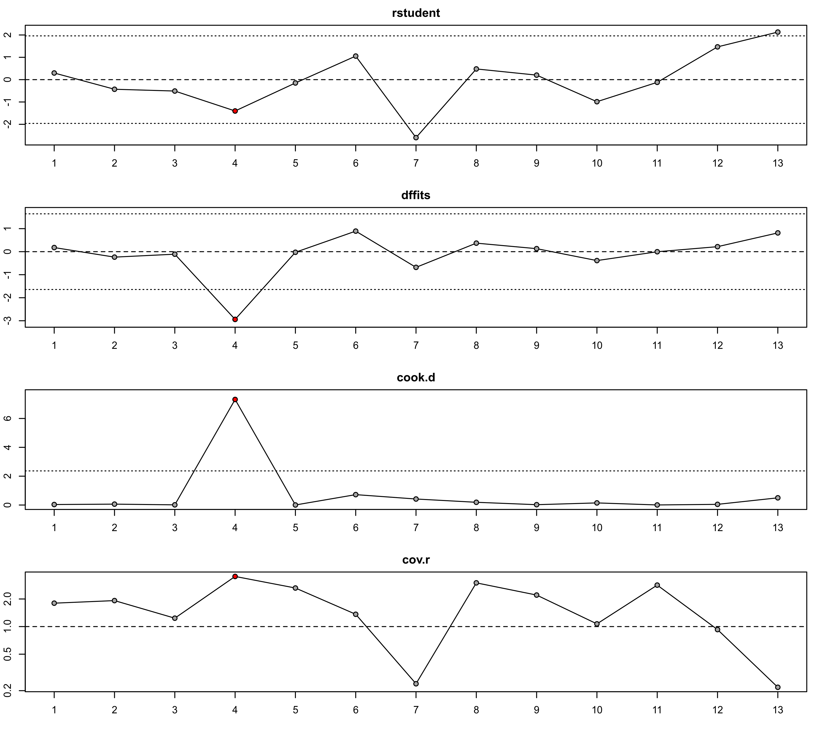
TRUE). Can also be a vector of up to 8 integers to specify which plots to draw. See ‘Details’ for the numbers corresponding to the various plots.- plotdfbs
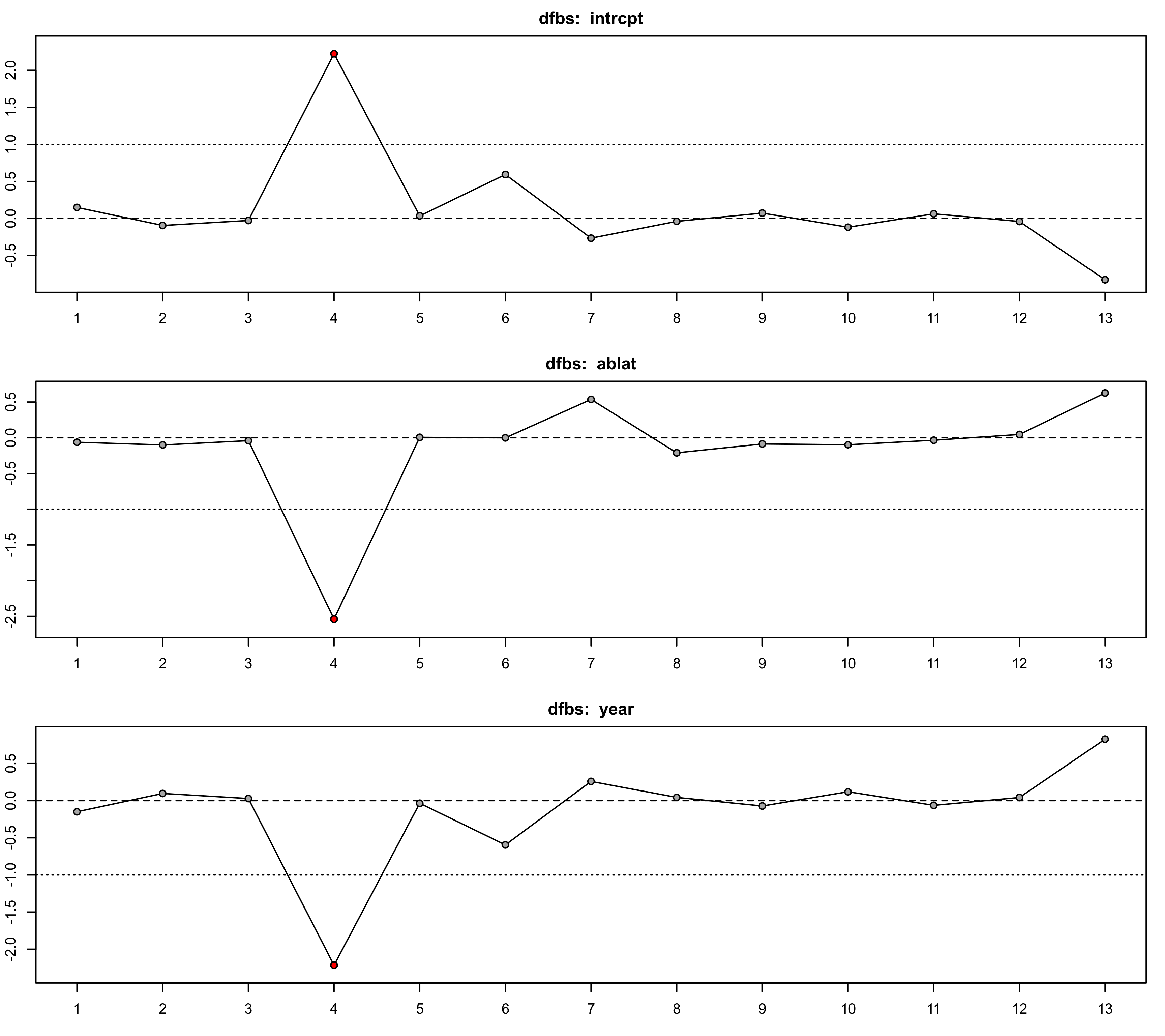
logical to specify whether the DFBETAS values should be plotted (the default is
FALSE). Can also be a vector of integers to specify for which coefficient(s) to plot the DFBETAS values.- dfbsnew
logical to specify whether a new device should be opened for plotting the DFBETAS values (the default is
FALSE).- logcov
logical to specify whether the covariance ratios should be plotted on a log scale (the default is
TRUE).- slab.style
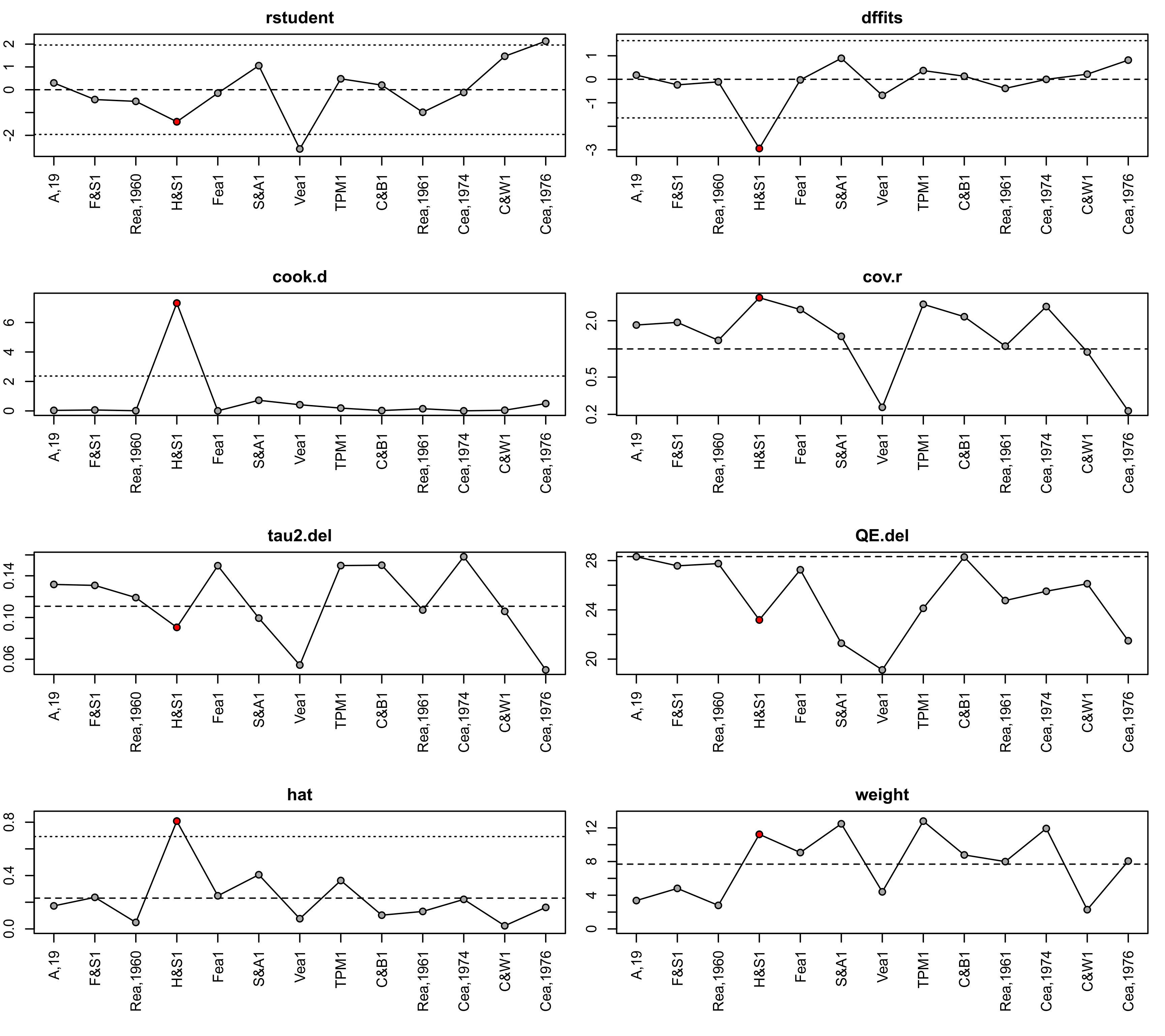
integer to specify the style of the x-axis labels: 1 = study number, 2 = study label, 3 = abbreviated study label. Note that study labels, even when abbreviated, may be too long to fit in the margins (see argument
marforparto adjust the margin sizes).- las
integer between 0 and 3 to specify the alignment of the axis labels (see
par). The most useful alternative to 0 is 3, so that the x-axis labels are drawn vertical to the axis.- pch
plotting symbol to use. By default, an open circle is used. See
pointsfor other options.- bg
optional character string to specify the background color of open plotting symbols. If unspecified, gray is used by default.
- bg.infl
optional character string to specify the background color when the point is considered influential. If unspecified, red is used by default.
- col.na
optional character string to specify the color for lines connecting two points with
NAvalues in between. If unspecified, a light shade of gray is used by default.- ...
other arguments.
Details
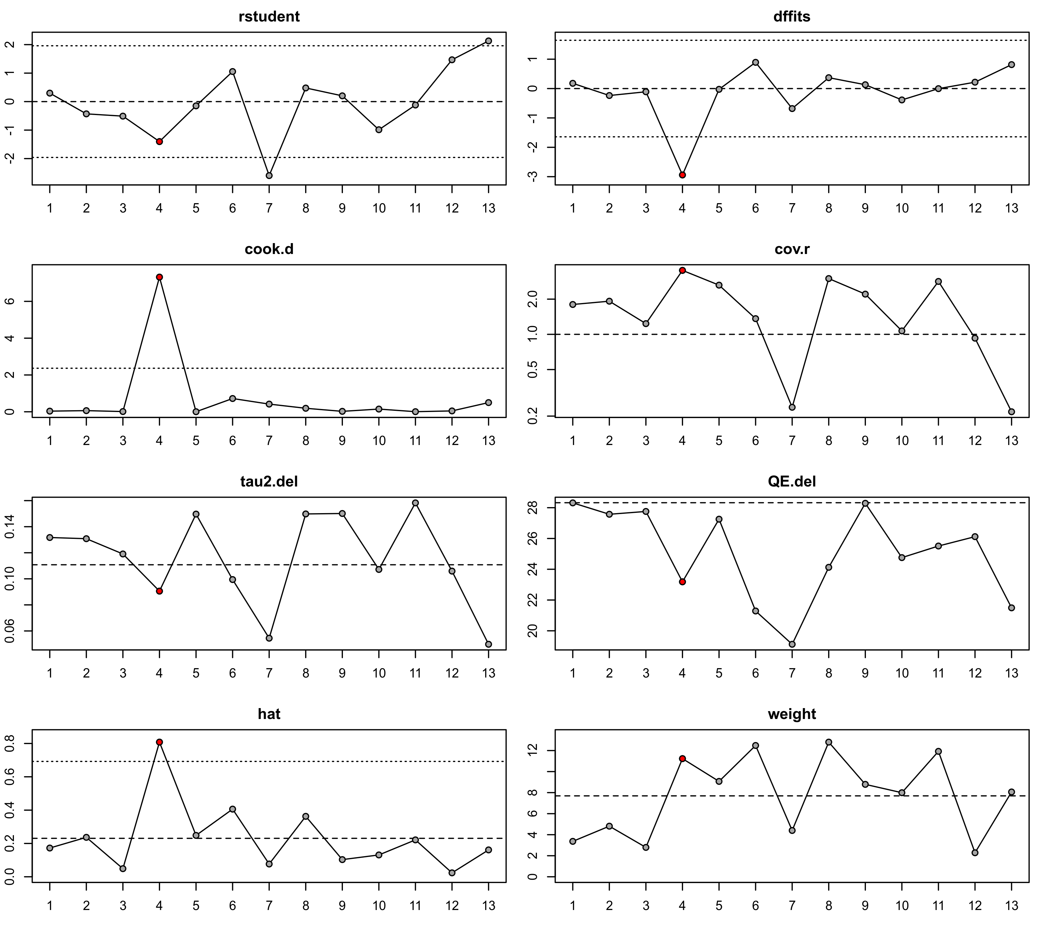
When plotinf=TRUE, the function plots the (1) externally standardized residuals, (2) DFFITS values, (3) Cook's distances, (4) covariance ratios, (5) leave-one-out \(\tau^2\) estimates, (6) leave-one-out (residual) heterogeneity test statistics, (7) hat values, and (8) weights. If plotdfbs=TRUE, the DFBETAS values are also plotted either after confirming the page change (if dfbsnew=FALSE) or on a separate device (if dfbsnew=TRUE).
A case (which is typically synonymous with study) may be considered to be ‘influential’ if at least one of the following is true:
The absolute DFFITS value is larger than \(3 \times \sqrt{p/(k-p)}\), where \(p\) is the number of model coefficients and \(k\) the number of cases.
The lower tail area of a chi-square distribution with \(p\) degrees of freedom cut off by the Cook's distance is larger than 50%.
The hat value is larger than \(3 \times (p/k)\).
Any DFBETAS value is larger than \(1\).
Cases which are considered influential with respect to any of these measures are indicated by the color specified for the bg.infl argument (the default is "red").
The cut-offs described above are indicated in the plot with horizontal reference lines. In addition, on the plot of the externally standardized residuals, horizontal reference lines are drawn at -1.96, 0, and 1.96. On the plot of the covariance ratios, a horizontal reference line is drawn at 1. On the plot of leave-one-out \(\tau^2\) estimates, a horizontal reference line is drawn at the \(\tau^2\) estimate based on all cases. On the plot of leave-one-out (residual) heterogeneity test statistics, horizontal reference lines are drawn at the test statistic based on all cases and at \(k-p\), the degrees of freedom of the test statistic. On the plot of the hat values, a horizontal reference line is drawn at \(p/k\). Since the sum of the hat values is equal to \(p\), the value \(p/k\) indicates equal hat values for all \(k\) cases. Finally, on the plot of weights, a horizontal reference line is drawn at \(100/k\), corresponding to the value for equal weights (in %) for all \(k\) cases. Note that all weights will automatically be equal to each other when using unweighted model fitting. Also, the hat values will be equal to the weights (except for their scaling) in models without moderators.
The chosen cut-offs are (somewhat) arbitrary. Substantively informed judgment should always be used when examining the influence of each case on the results.
References
Viechtbauer, W. (2010). Conducting meta-analyses in R with the metafor package. Journal of Statistical Software, 36(3), 1–48. https://doi.org/10.18637/jss.v036.i03
Viechtbauer, W., & Cheung, M. W.-L. (2010). Outlier and influence diagnostics for meta-analysis. Research Synthesis Methods, 1(2), 112–125. https://doi.org/10.1002/jrsm.11
See also
influence for the function to compute the various model diagnostics.
Examples
### calculate log risk ratios and corresponding sampling variances
dat <- escalc(measure="RR", ai=tpos, bi=tneg, ci=cpos, di=cneg,
              data=dat.bcg, slab=paste(author, year, sep=", "))

### fit mixed-effects model with absolute latitude and publication year as moderators
res <- rma(yi, vi, mods = ~ ablat + year, data=dat)

### compute the diagnostics
inf <- influence(res)

### plot the values
plot(inf)


### show the abbreviated study labels on the x-axis
op <- par(mar=c(8,4,4,2))
plot(inf, slab.style=3, las=3)

par(op)

### select which plots to show
plot(inf, plotinf=1:4)


### plot the DFBETAS values
plot(inf, plotinf=FALSE, plotdfbs=TRUE)
