Plot of Likelihoods for Individual Studies
llplot.RdFunction to plot the likelihood of a certain parameter corresponding to an effect size or outcome measure given the study data.
llplot(measure, yi, vi, sei, ai, bi, ci, di, n1i, n2i, data, subset, drop00=TRUE,
       xvals=1000, xlim, ylim, xlab, ylab, scale=TRUE,
       lty, lwd, col, level=99.99, refline=0, ...)
Arguments
- measure
a character string to specify for which effect size or outcome measure the likelihoods should be calculated. See ‘Details’ for possible options and how the data should then be specified.
- yi
vector with the observed effect sizes or outcomes.
- vi
vector with the corresponding sampling variances.
- sei
vector with the corresponding standard errors.
- ai
vector to specify the \(2 \times 2\) table frequencies (upper left cell).
- bi
vector to specify the \(2 \times 2\) table frequencies (upper right cell).
- ci
vector to specify the \(2 \times 2\) table frequencies (lower left cell).
- di
vector to specify the \(2 \times 2\) table frequencies (lower right cell).
- n1i
vector to specify the group sizes or row totals (first group/row).
- n2i
vector to specify the group sizes or row totals (second group/row).
- data
optional data frame containing the variables given to the arguments above.
- subset
optional (logical or numeric) vector to specify the subset of studies that should be included in the plot.
- drop00
logical to specify whether studies with no cases (or only cases) in both groups should be dropped. See ‘Details’.
- xvals
integer to specify for how many distinct values the likelihood should be evaluated.
- xlim
x-axis limits. If unspecified, the function sets the x-axis limits to some sensible values.
- ylim
y-axis limits. If unspecified, the function sets the y-axis limits to some sensible values.
- xlab
title for the x-axis. If unspecified, the function sets an appropriate axis title.
- ylab
title for the y-axis. If unspecified, the function sets an appropriate axis title.
- scale
logical to specify whether the likelihood values should be scaled, so that the total area under each curve is (approximately) equal to 1.
- lty
the line types (either a single value or a vector of length \(k\)). If unspecified, the function sets the line types according to some characteristics of the likelihood function. See ‘Details’.
- lwd
the line widths (either a single value or a vector of length \(k\)). If unspecified, the function sets the widths according to the sampling variances (so that the line is thicker for more precise studies and vice-versa).
- col
the line colors (either a single value or a vector of length \(k\)). If unspecified, the function uses various shades of gray according to the sampling variances (so that darker shades are used for more precise studies and vice-versa).
- level
numeric value between 0 and 100 to specify the plotting limits for each likelihood line in terms of the confidence interval (the default is 99.99).
- refline
numeric value to specify the location of the vertical ‘reference’ line (the default is 0). The line can be suppressed by setting this argument to
NA.- ...
other arguments.
Details
At the moment, the function only accepts measure="GEN" or measure="OR".
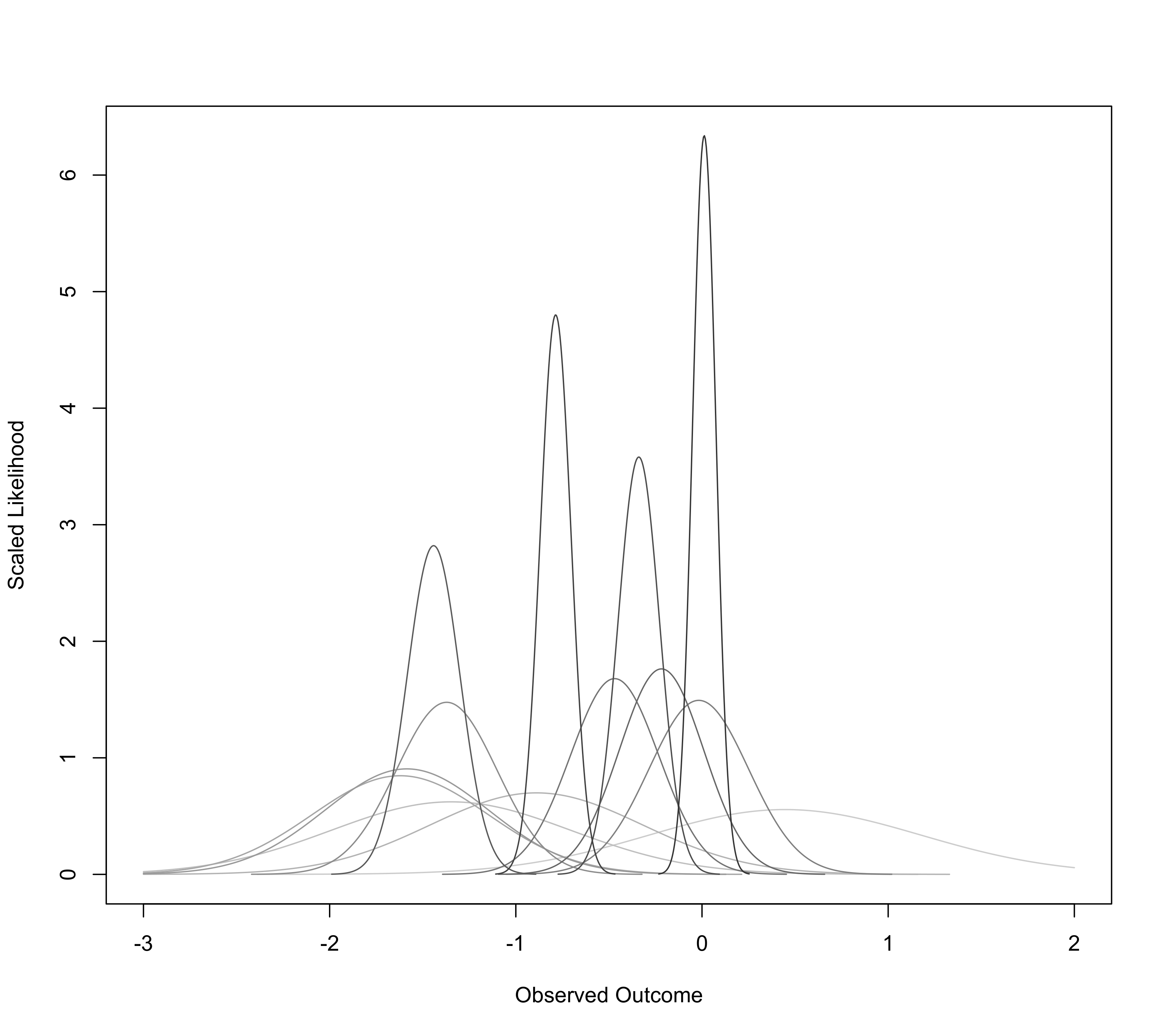
For measure="GEN", one must specify arguments yi for the observed effect sizes or outcomes and vi for the corresponding sampling variances (instead of specifying vi, one can specify the standard errors via the sei argument). The function then plots the likelihood of the true effect size or outcome based on a normal sampling distribution with observed outcome as given by yi and variance as given by vi for each study.
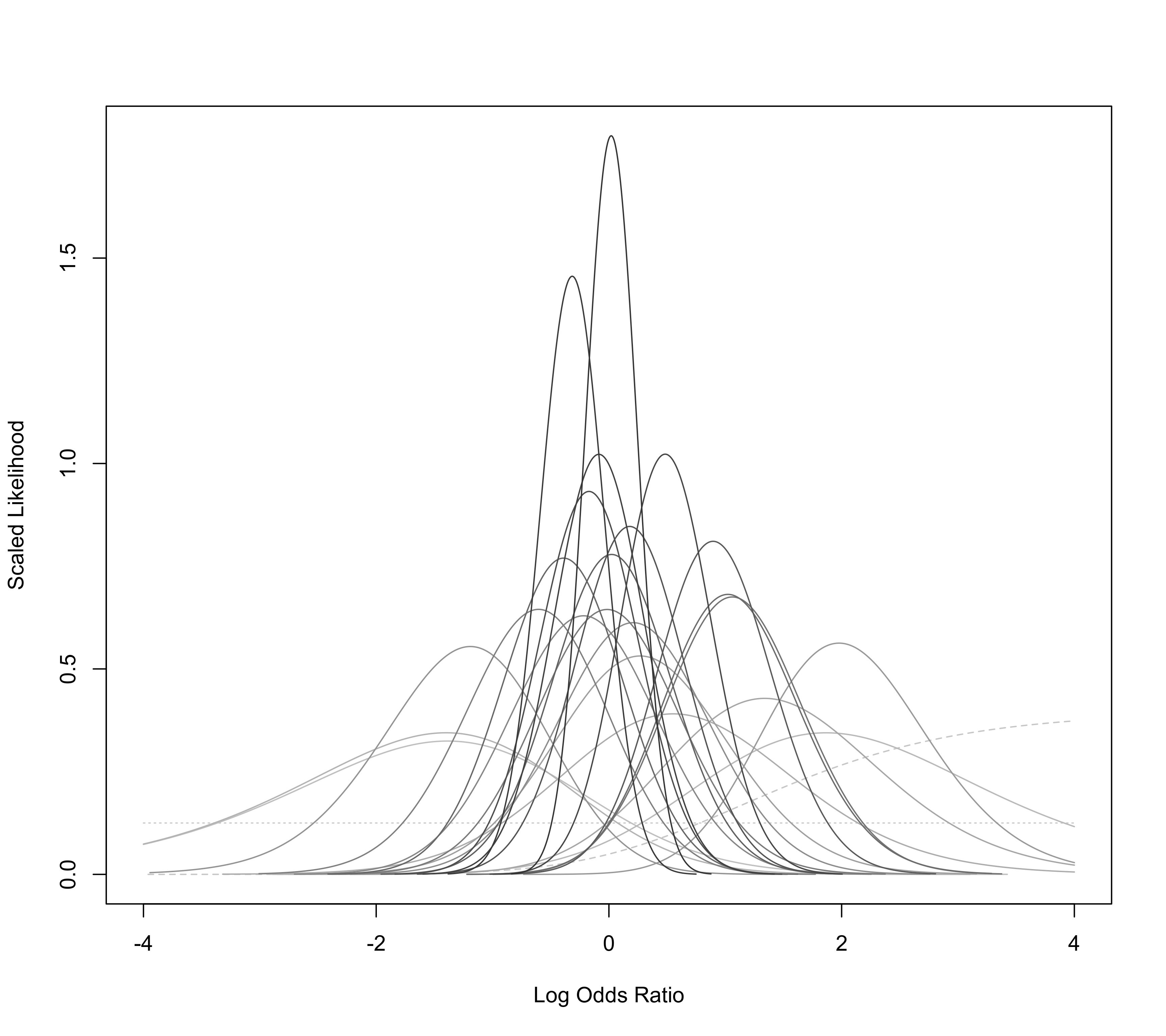
For measure="OR", one must specify arguments ai, bi, ci, and di, which denote the cell frequencies of the \(2 \times 2\) tables. Alternatively, one can specify ai, ci, n1i, and n2i. See escalc function for more details. The function then plots the likelihood of the true log odds ratio based on the non-central hypergeometric distribution for each \(2 \times 2\) table. Since studies with no cases (or only cases) in both groups have a flat likelihood and are not informative about the odds ratio, they are dropped by default (i.e., drop00=TRUE) and are hence not drawn (if drop00=FALSE, these likelihoods are indicated by dotted lines). For studies that have a single zero count, the MLE of the odds ratio is infinite and these likelihoods are indicated by dashed lines.
References
van Houwelingen, H. C., Zwinderman, K. H., & Stijnen, T. (1993). A bivariate approach to meta-analysis. Statistics in Medicine, 12(24), 2273–2284. https://doi.org/10.1002/sim.4780122405
Viechtbauer, W. (2010). Conducting meta-analyses in R with the metafor package. Journal of Statistical Software, 36(3), 1–48. https://doi.org/10.18637/jss.v036.i03
See also
Examples
### calculate log risk ratios and corresponding sampling variances
dat <- escalc(measure="RR", ai=tpos, bi=tneg, ci=cpos, di=cneg, data=dat.bcg)

### draw likelihoods
llplot(measure="GEN", yi=yi, vi=vi, data=dat, lwd=1, refline=NA, xlim=c(-3,2))


### create plot (Figure 2 in van Houwelingen, Zwinderman, & Stijnen, 1993)
llplot(measure="OR", ai=b.xci, n1i=nci, ci=b.xti, n2i=nti, data=dat.collins1985a,
       lwd=1, refline=NA, xlim=c(-4,4), drop00=FALSE)
#> Warning: 2 studies with NAs omitted from plotting.
