Add Polygons to Forest Plots (Method for 'rma' Objects)

Function to add a polygon to a forest plot showing the pooled estimate with corresponding confidence interval based on an object of class "rma".

# S3 method for class 'rma'
addpoly(x, row=-2, level=x$level, annotate,
        addpred=FALSE, predstyle, predlim, digits, width, mlab,
        transf, atransf, targs, efac, col, border, lty, fonts, cex, ...)

Arguments

x: an object of class "rma".
row: numeric value to specify the row (or more generally, the position) for plotting the polygon (the default is -2).
level: numeric value between 0 and 100 to specify the confidence interval level (see here for details). The default is to take the value from the object.
annotate: optional logical to specify whether annotations for the pooled estimate should be added to the plot.
addpred: logical to specify whether the prediction interval should be added to the plot (the default is FALSE).
predstyle: character string to specify the style of the prediction interval (either "line", "bar", "shade", or "dist"). Can be abbreviated. Setting this argument automatically sets addpred=TRUE.
predlim: optional argument to specify the limits of the prediction distribution when predstyle="dist".
digits: optional integer to specify the number of decimal places to which the annotations should be rounded.
width: optional integer to manually adjust the width of the columns for the annotations.
mlab: optional character string giving a label for the pooled estimate. If unspecified, the function sets a default label.
transf: optional argument to specify a function to transform the pooled estimate and confidence interval bounds (e.g., transf=exp; see also transf).
atransf: optional argument to specify a function to transform the annotations (e.g., atransf=exp; see also transf).
targs: optional arguments needed by the function specified via transf or atransf.
efac: optional vertical expansion factor for the polygon.
col: optional character string to specify the color of the polygon.
border: optional character string to specify the border color of the polygon.
lty: optional argument to specify the line type for the prediction interval.
fonts: optional character string to specify the font for the label and annotations.
cex: optional symbol expansion factor.
...: other arguments.

Details

The function can be used to add a four-sided polygon, sometimes called a summary ‘diamond’, to an existing forest plot created with the forest function. The polygon shows the pooled estimate (with its confidence interval bounds) based on an equal- or a random-effects model. Using this function, pooled estimates based on different types of models can be shown in the same plot. Also, pooled estimates based on a subgrouping of the studies can be added to the plot this way. See ‘Examples’.

If unspecified, arguments annotate, digits, width, transf, atransf, targs, efac (only if the forest plot was created with forest.rma), fonts, cex, annosym, and textpos are automatically set equal to the same values that were used when creating the forest plot.

Author

Wolfgang Viechtbauer (wvb@metafor-project.org, https://www.metafor-project.org).

References

Viechtbauer, W. (2010). Conducting meta-analyses in R with the metafor package. Journal of Statistical Software, 36(3), 1–48. https://doi.org/10.18637/jss.v036.i03

Examples

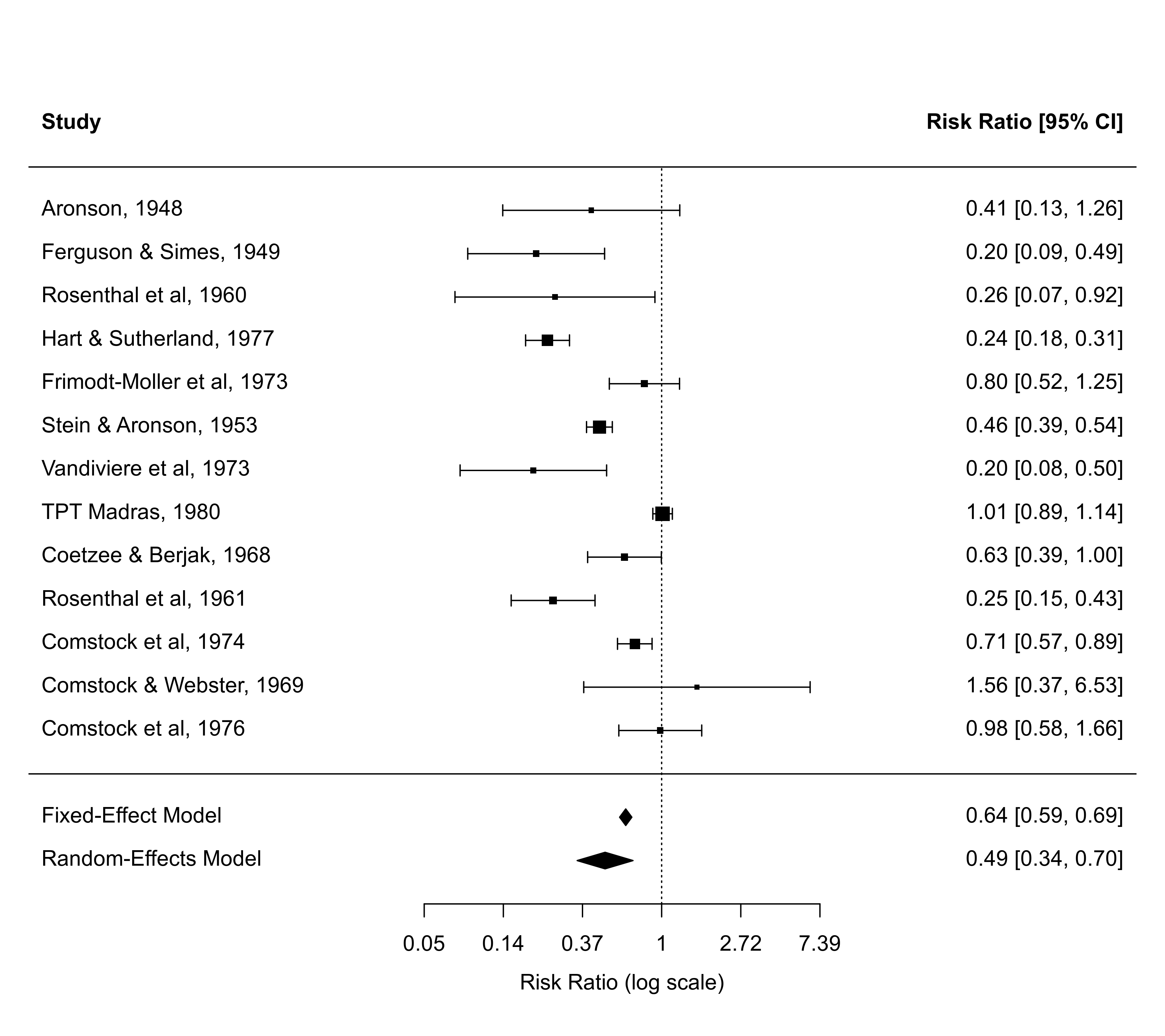
### meta-analysis of the log risk ratios using the Mantel-Haenszel method
res <- rma.mh(measure="RR", ai=tpos, bi=tneg, ci=cpos, di=cneg, data=dat.bcg,
              slab=paste(author, year, sep=", "))

### forest plot of the observed risk ratios with the pooled estimate
forest(res, atransf=exp, xlim=c(-8,6), ylim=c(-3,16))

### meta-analysis of the log risk ratios using a random-effects model
res <- rma(measure="RR", ai=tpos, bi=tneg, ci=cpos, di=cneg, data=dat.bcg)

### add the pooled estimate from the random-effects model to the forest plot
addpoly(res)


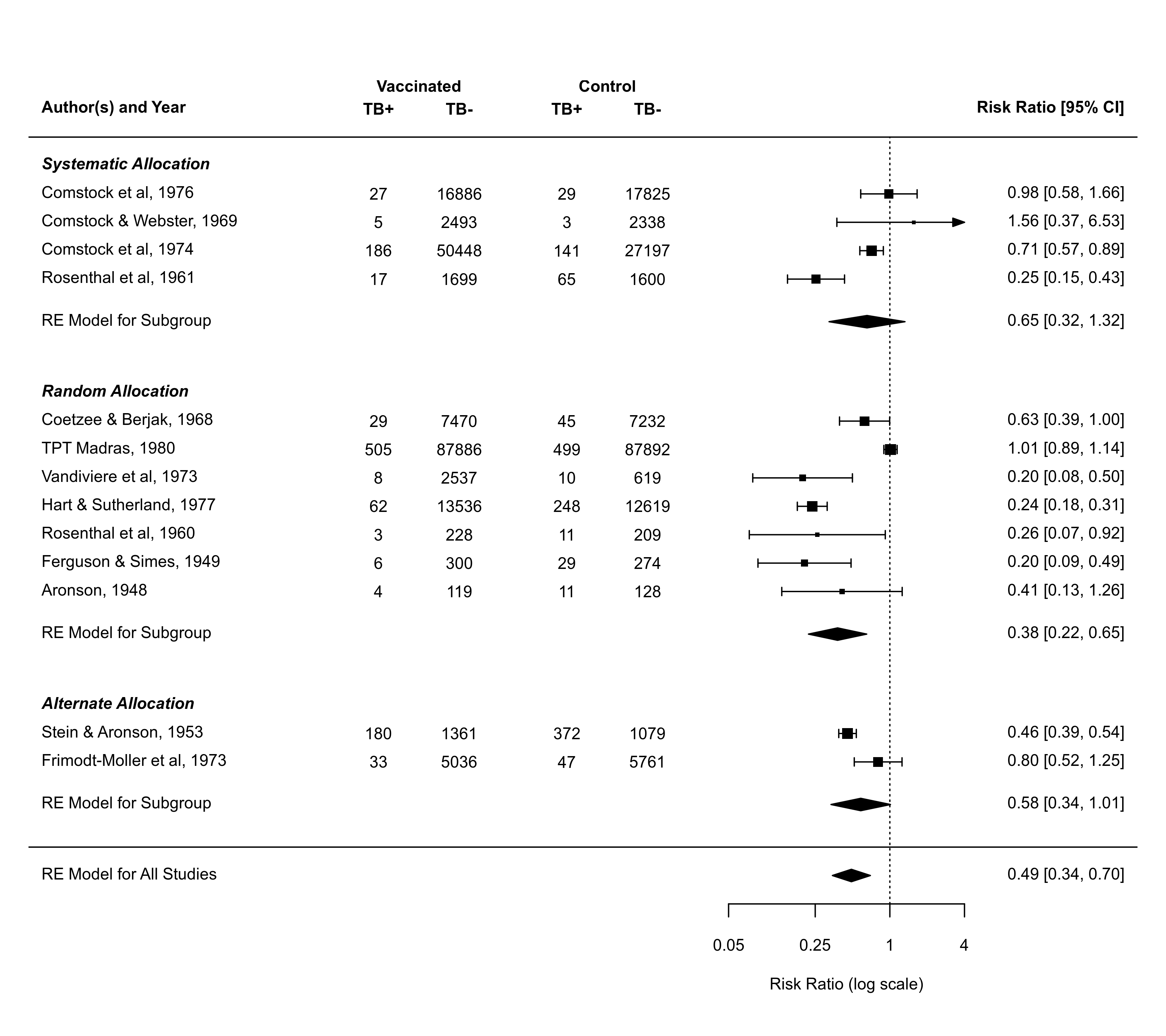
### forest plot with subgrouping of studies and summaries per subgroup
dat <- escalc(measure="RR", ai=tpos, bi=tneg, ci=cpos, di=cneg, data=dat.bcg,
              slab=paste(author, year, sep=", "))
res <- rma(yi, vi, data=dat)
tmp <- forest(res, xlim=c(-16, 4.6), at=log(c(0.05, 0.25, 1, 4)), atransf=exp,
              ilab=cbind(tpos, tneg, cpos, cneg), ilab.lab=c("TB+","TB-","TB+","TB-"),
              ilab.xpos=c(-9.5,-8,-6,-4.5), cex=0.75, ylim=c(-2, 27), order=alloc,
              rows=c(3:4,9:15,20:23), mlab="RE Model for All Studies",
              header="Author(s) and Year")
op <- par(cex=tmp$cex)
text(c(-8.75,-5.25), tmp$ylim[2]-0.2, c("Vaccinated", "Control"), font=2)
text(-16, c(24,16,5), c("Systematic Allocation", "Random Allocation",
                        "Alternate Allocation"), font=4, pos=4)
par(op)
res <- rma(yi, vi, data=dat, subset=(alloc=="systematic"))
addpoly(res, row=18.5, mlab="RE Model for Subgroup")
res <- rma(yi, vi, data=dat, subset=(alloc=="random"))
addpoly(res, row=7.5, mlab="RE Model for Subgroup")
res <- rma(yi, vi, data=dat, subset=(alloc=="alternate"))
addpoly(res, row=1.5, mlab="RE Model for Subgroup")