Studies on the Effectiveness of Counseling for Smoking Cessation
dat.hasselblad1998.RdResults from 24 studies on the effectiveness of various counseling types for smoking cessation.
dat.hasselblad1998Format
The data frame contains the following columns:
| id | numeric | id number for each treatment arm |
| study | numeric | study id number |
| authors | character | study author(s) |
| year | numeric | publication year |
| trt | character | intervention group |
| xi | numeric | number of individuals abstinent |
| ni | numeric | number of individuals in group |
Details
The dataset includes the results from 24 studies on the effectiveness of various counseling types for smoking cessation (i.e., self-help, individual counseling, group counseling, and no contact). The dataset indicates the total number of individuals within each study arm and the number that were abstinent from 6 to 12 months. The majority of the studies compared two interventions types against each other, while 2 studies compared three types against each other simultaneously.
The data can be used for a ‘network meta-analysis’ (also called a ‘mixed treatment comparison’). The code below shows how such an analysis can be conducted using an arm-based and a contrast-based model (see Salanti et al., 2008, for more details).
Source
Hasselblad, V. (1998). Meta-analysis of multitreatment studies. Medical Decision Making, 18(1), 37–43. https://doi.org/10.1177/0272989X9801800110
References
Gleser, L. J., & Olkin, I. (2009). Stochastically dependent effect sizes. In H. Cooper, L. V. Hedges, & J. C. Valentine (Eds.), The handbook of research synthesis and meta-analysis (2nd ed., pp. 357–376). New York: Russell Sage Foundation.
Law, M., Jackson, D., Turner, R., Rhodes, K., & Viechtbauer, W. (2016). Two new methods to fit models for network meta-analysis with random inconsistency effects. BMC Medical Research Methodology, 16, 87. https://doi.org/10.1186/s12874-016-0184-5
Salanti, G., Higgins, J. P. T., Ades, A. E., & Ioannidis, J. P. A. (2008). Evaluation of networks of randomized trials. Statistical Methods in Medical Research, 17(3), 279–301. https://doi.org/10.1177/0962280207080643
Concepts
medicine, psychology, smoking, odds ratios, network meta-analysis
Examples
### copy data into 'dat' and examine data
dat <- dat.hasselblad1998
dat
#> id study authors year trt xi ni
#> 1 1 1 Reid et al. 1974 no_contact 75 731
#> 2 2 1 Reid et al. 1974 ind_counseling 363 714
#> 3 3 2 Cottraux et al. 1983 no_contact 9 140
#> 4 4 2 Cottraux et al. 1983 ind_counseling 23 140
#> 5 5 2 Cottraux et al. 1983 grp_counseling 10 138
#> 6 6 3 Slama et al. 1990 no_contact 2 106
#> 7 7 3 Slama et al. 1990 ind_counseling 9 205
#> 8 8 4 Jamrozik et al. 1984 no_contact 58 549
#> 9 9 4 Jamrozik et al. 1984 ind_counseling 237 1561
#> 10 10 5 Rabkin et al. 1984 no_contact 0 33
#> 11 11 5 Rabkin et al. 1984 ind_counseling 9 48
#> 12 12 6 Decker and Evans 1989 self_help 20 49
#> 13 13 6 Decker and Evans 1989 ind_counseling 16 43
#> 14 14 7 Richmond et al. 1986 no_contact 3 100
#> 15 15 7 Richmond et al. 1986 ind_counseling 31 98
#> 16 16 8 Leung 1991 no_contact 1 31
#> 17 17 8 Leung 1991 ind_counseling 26 95
#> 18 18 9 Mothersill et al. 1988 self_help 11 78
#> 19 19 9 Mothersill et al. 1988 ind_counseling 12 85
#> 20 20 9 Mothersill et al. 1988 grp_counseling 29 170
#> 21 21 10 Langford et al. 1983 no_contact 6 39
#> 22 22 10 Langford et al. 1983 ind_counseling 17 77
#> 23 23 11 Gritz et al. 1992 no_contact 79 702
#> 24 24 11 Gritz et al. 1992 self_help 77 694
#> 25 25 12 Campbell et al. 1986 no_contact 18 671
#> 26 26 12 Campbell et al. 1986 self_help 21 535
#> 27 27 13 Sanders et al. 1989 no_contact 64 642
#> 28 28 13 Sanders et al. 1989 ind_counseling 107 761
#> 29 29 14 Hilleman et al. 1993 ind_counseling 12 76
#> 30 30 14 Hilleman et al. 1993 grp_counseling 20 74
#> 31 31 15 Gillams et al. 1984 ind_counseling 9 55
#> 32 32 15 Gillams et al. 1984 grp_counseling 3 26
#> 33 33 16 Mogielnicki et al. 1986 self_help 7 66
#> 34 34 16 Mogielnicki et al. 1986 grp_counseling 32 127
#> 35 35 17 Page et al. 1986 no_contact 5 62
#> 36 36 17 Page et al. 1986 ind_counseling 8 90
#> 37 37 18 Vetter and Ford 1990 no_contact 20 234
#> 38 38 18 Vetter and Ford 1990 ind_counseling 34 237
#> 39 39 19 Williams and Hall 1988 no_contact 0 20
#> 40 40 19 Williams and Hall 1988 grp_counseling 9 20
#> 41 41 20 Pallonen et al. 1994 no_contact 8 116
#> 42 42 20 Pallonen et al. 1994 self_help 19 149
#> 43 43 21 Russell et al. 1983 no_contact 95 1107
#> 44 44 21 Russell et al. 1983 ind_counseling 143 1031
#> 45 45 22 Stewart and Rosser 1982 no_contact 15 187
#> 46 46 22 Stewart and Rosser 1982 ind_counseling 36 504
#> 47 47 23 Russell et al. 1979 no_contact 78 584
#> 48 48 23 Russell et al. 1979 ind_counseling 73 675
#> 49 49 24 Kendrick et al. 1995 no_contact 69 1177
#> 50 50 24 Kendrick et al. 1995 ind_counseling 54 888
### load metafor package
library(metafor)
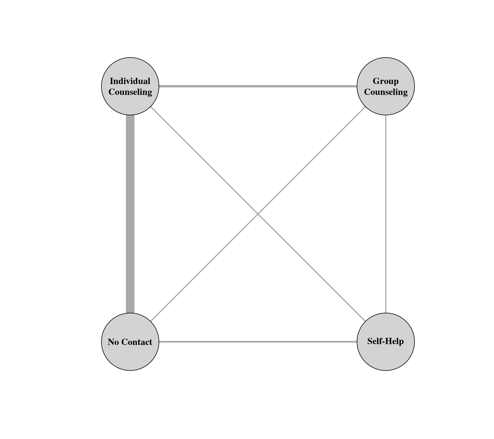
### create network graph ('igraph' package must be installed)
library(igraph, warn.conflicts=FALSE)
pairs <- data.frame(do.call(rbind,
sapply(split(dat$trt, dat$study), function(x) t(combn(x,2)))), stringsAsFactors=FALSE)
lvls <- c("no_contact", "self_help", "ind_counseling", "grp_counseling")
pairs$X1 <- factor(pairs$X1, levels=lvls)
pairs$X2 <- factor(pairs$X2, levels=lvls)
tab <- table(pairs[,1], pairs[,2])
tab # adjacency matrix
#>
#> no_contact self_help ind_counseling grp_counseling
#> no_contact 0 3 15 2
#> self_help 0 0 2 2
#> ind_counseling 0 0 0 4
#> grp_counseling 0 0 0 0
g <- graph_from_adjacency_matrix(tab, mode = "plus", weighted=TRUE, diag=FALSE)
vertex_attr(g, "name") <- c("No Contact", "Self-Help",
"Individual\nCounseling", "Group\nCounseling")
plot(g, edge.curved=FALSE, edge.width=E(g)$weight, layout=layout_on_grid,
vertex.size=45, vertex.color="lightgray", vertex.label.color="black", vertex.label.font=2)
 ### calculate log odds for each study arm
dat <- escalc(measure="PLO", xi=xi, ni=ni, add=1/2, to="all", data=dat)
dat
#>
#> id study authors year trt xi ni yi vi
#> 1 1 1 Reid et al. 1974 no_contact 75 731 -2.1628 0.0148
#> 2 2 1 Reid et al. 1974 ind_counseling 363 714 0.0336 0.0056
#> 3 3 2 Cottraux et al. 1983 no_contact 9 140 -2.6277 0.1129
#> 4 4 2 Cottraux et al. 1983 ind_counseling 23 140 -1.6094 0.0511
#> 5 5 2 Cottraux et al. 1983 grp_counseling 10 138 -2.5046 0.1030
#> 6 6 3 Slama et al. 1990 no_contact 2 106 -3.7329 0.4096
#> 7 7 3 Slama et al. 1990 ind_counseling 9 205 -3.0294 0.1104
#> 8 8 4 Jamrozik et al. 1984 no_contact 58 549 -2.1284 0.0191
#> 9 9 4 Jamrozik et al. 1984 ind_counseling 237 1561 -1.7186 0.0050
#> 10 10 5 Rabkin et al. 1984 no_contact 0 33 -4.2047 2.0299
#> 11 11 5 Rabkin et al. 1984 ind_counseling 9 48 -1.4250 0.1306
#> 12 12 6 Decker and Evans 1989 self_help 20 49 -0.3640 0.0827
#> 13 13 6 Decker and Evans 1989 ind_counseling 16 43 -0.5108 0.0970
#> 14 14 7 Richmond et al. 1986 no_contact 3 100 -3.3271 0.2960
#> 15 15 7 Richmond et al. 1986 ind_counseling 31 98 -0.7621 0.0466
#> 16 16 8 Leung 1991 no_contact 1 31 -3.0123 0.6995
#> 17 17 8 Leung 1991 ind_counseling 26 95 -0.9642 0.0521
#> 18 18 9 Mothersill et al. 1988 self_help 11 78 -1.7698 0.1018
#> 19 19 9 Mothersill et al. 1988 ind_counseling 12 85 -1.7716 0.0936
#> 20 20 9 Mothersill et al. 1988 grp_counseling 29 170 -1.5679 0.0410
#> 21 21 10 Langford et al. 1983 no_contact 6 39 -1.6397 0.1837
#> 22 22 10 Langford et al. 1983 ind_counseling 17 77 -1.2404 0.0737
#> 23 23 11 Gritz et al. 1992 no_contact 79 702 -2.0596 0.0142
#> 24 24 11 Gritz et al. 1992 self_help 77 694 -2.0754 0.0145
#> 25 25 12 Campbell et al. 1986 no_contact 18 671 -3.5646 0.0556
#> 26 26 12 Campbell et al. 1986 self_help 21 535 -3.1751 0.0485
#> 27 27 13 Sanders et al. 1989 no_contact 64 642 -2.1938 0.0172
#> 28 28 13 Sanders et al. 1989 ind_counseling 107 761 -1.8064 0.0108
#> 29 29 14 Hilleman et al. 1993 ind_counseling 12 76 -1.6409 0.0955
#> 30 30 14 Hilleman et al. 1993 grp_counseling 20 74 -0.9778 0.0671
#> 31 31 15 Gillams et al. 1984 ind_counseling 9 55 -1.5882 0.1268
#> 32 32 15 Gillams et al. 1984 grp_counseling 3 26 -1.9042 0.3283
#> 33 33 16 Mogielnicki et al. 1986 self_help 7 66 -2.0711 0.1501
#> 34 34 16 Mogielnicki et al. 1986 grp_counseling 32 127 -1.0779 0.0412
#> 35 35 17 Page et al. 1986 no_contact 5 62 -2.3470 0.1992
#> 36 36 17 Page et al. 1986 ind_counseling 8 90 -2.2727 0.1298
#> 37 37 18 Vetter and Ford 1990 no_contact 20 234 -2.3479 0.0534
#> 38 38 18 Vetter and Ford 1990 ind_counseling 34 237 -1.7747 0.0339
#> 39 39 19 Williams and Hall 1988 no_contact 0 20 -3.7136 2.0488
#> 40 40 19 Williams and Hall 1988 grp_counseling 9 20 -0.1911 0.1922
#> 41 41 20 Pallonen et al. 1994 no_contact 8 116 -2.5467 0.1269
#> 42 42 20 Pallonen et al. 1994 self_help 19 149 -1.9010 0.0589
#> 43 43 21 Russell et al. 1983 no_contact 95 1107 -2.3611 0.0115
#> 44 44 21 Russell et al. 1983 ind_counseling 143 1031 -1.8232 0.0081
#> 45 45 22 Stewart and Rosser 1982 no_contact 15 187 -2.4096 0.0703
#> 46 46 22 Stewart and Rosser 1982 ind_counseling 36 504 -2.5522 0.0295
#> 47 47 23 Russell et al. 1979 no_contact 78 584 -1.8644 0.0147
#> 48 48 23 Russell et al. 1979 ind_counseling 73 675 -2.1038 0.0153
#> 49 49 24 Kendrick et al. 1995 no_contact 69 1177 -2.7694 0.0153
#> 50 50 24 Kendrick et al. 1995 ind_counseling 54 888 -2.7286 0.0195
#>
### convert trt variable to factor with desired ordering of levels
dat$trt <- factor(dat$trt, levels=c("no_contact", "self_help", "ind_counseling", "grp_counseling"))
### add a space before each level (this makes the output a bit more legible)
levels(dat$trt) <- paste0(" ", levels(dat$trt))
### network meta-analysis using an arm-based model with fixed study effects
### by setting rho=1/2, tau^2 reflects the amount of heterogeneity for all treatment comparisons
res <- rma.mv(yi, vi, mods = ~ 0 + factor(study) + trt,
random = ~ trt | study, rho=1/2, data=dat, btt="trt")
res
#>
#> Multivariate Meta-Analysis Model (k = 50; method: REML)
#>
#> Variance Components:
#>
#> outer factor: study (nlvls = 24)
#> inner factor: trt (nlvls = 4)
#>
#> estim sqrt fixed
#> tau^2 0.4324 0.6575 no
#> rho 0.5000 yes
#>
#> Test for Residual Heterogeneity:
#> QE(df = 23) = 202.3334, p-val < .0001
#>
#> Test of Moderators (coefficients 25:27):
#> QM(df = 3) = 14.2278, p-val = 0.0026
#>
#> Model Results:
#>
#> estimate se zval pval ci.lb ci.ub
#> factor(study)1 -1.3925 0.5820 -2.3926 0.0167 -2.5333 -0.2518 *
#> factor(study)2 -2.7302 0.5842 -4.6731 <.0001 -3.8753 -1.5851 ***
#> factor(study)3 -3.7217 0.6681 -5.5703 <.0001 -5.0312 -2.4121 ***
#> factor(study)4 -2.2710 0.5829 -3.8958 <.0001 -3.4136 -1.1285 ***
#> factor(study)5 -2.3914 0.7374 -3.2430 0.0012 -3.8367 -0.9461 **
#> factor(study)6 -0.9698 0.6421 -1.5104 0.1309 -2.2284 0.2887
#> factor(study)7 -2.0855 0.6369 -3.2744 0.0011 -3.3339 -0.8372 **
#> factor(study)8 -1.9592 0.6674 -2.9357 0.0033 -3.2672 -0.6512 **
#> factor(study)9 -2.3487 0.6032 -3.8936 <.0001 -3.5310 -1.1664 ***
#> factor(study)10 -1.8062 0.6296 -2.8688 0.0041 -3.0402 -0.5722 **
#> factor(study)11 -2.2618 0.5978 -3.7835 0.0002 -3.4334 -1.0901 ***
#> factor(study)12 -3.5643 0.6139 -5.8058 <.0001 -4.7675 -2.3610 ***
#> factor(study)13 -2.3454 0.5836 -4.0188 <.0001 -3.4892 -1.2015 ***
#> factor(study)14 -2.0624 0.6492 -3.1767 0.0015 -3.3348 -0.7899 **
#> factor(study)15 -2.4575 0.6868 -3.5781 0.0003 -3.8037 -1.1114 ***
#> factor(study)16 -2.1438 0.6707 -3.1964 0.0014 -3.4583 -0.8293 **
#> factor(study)17 -2.6810 0.6448 -4.1581 <.0001 -3.9447 -1.4173 ***
#> factor(study)18 -2.4066 0.5964 -4.0353 <.0001 -3.5755 -1.2377 ***
#> factor(study)19 -1.4441 0.8108 -1.7811 0.0749 -3.0331 0.1450 .
#> factor(study)20 -2.4041 0.6331 -3.7974 0.0001 -3.6450 -1.1633 ***
#> factor(study)21 -2.4359 0.5817 -4.1877 <.0001 -3.5760 -1.2958 ***
#> factor(study)22 -2.8559 0.5991 -4.7667 <.0001 -4.0301 -1.6816 ***
#> factor(study)23 -2.3268 0.5838 -3.9857 <.0001 -3.4710 -1.1826 ***
#> factor(study)24 -3.0893 0.5847 -5.2836 <.0001 -4.2353 -1.9433 ***
#> trt self_help 0.3888 0.3221 1.2070 0.2274 -0.2426 1.0202
#> trt ind_counseling 0.6864 0.1904 3.6055 0.0003 0.3133 1.0596 ***
#> trt grp_counseling 0.8438 0.3641 2.3176 0.0205 0.1302 1.5574 *
#>
#> ---
#> Signif. codes: 0 ‘***’ 0.001 ‘**’ 0.01 ‘*’ 0.05 ‘.’ 0.1 ‘ ’ 1
#>
### all pairwise odds ratios of interventions versus no contact
predict(res, newmods=cbind(matrix(0, nrow=3, ncol=24), diag(3)),
intercept=FALSE, transf=exp, digits=2)
#> Warning: Arguments 'intercept' ignored when 'newmods' includes 'p' columns.
#>
#> pred ci.lb ci.ub pi.lb pi.ub
#> 1 1.48 0.78 2.77 0.35 6.20
#> 2 1.99 1.37 2.89 0.52 7.60
#> 3 2.33 1.14 4.75 0.53 10.14
#>
### all pairwise odds ratios comparing interventions (ic vs sh, gc vs sh, and gc vs ic)
predict(res, newmods=cbind(matrix(0, nrow=3, ncol=24), rbind(c(-1,1,0), c(-1,0,1), c(0,-1,1))),
intercept=FALSE, transf=exp, digits=2)
#> Warning: Arguments 'intercept' ignored when 'newmods' includes 'p' columns.
#>
#> pred ci.lb ci.ub pi.lb pi.ub
#> 1 1.35 0.70 2.58 0.32 5.71
#> 2 1.58 0.72 3.43 0.35 7.10
#> 3 1.17 0.59 2.30 0.27 5.02
#>
### forest plot of ORs of interventions versus no contact
forest(c(0,res$beta[25:27]), sei=c(0,res$se[25:27]), psize=1, xlim=c(-3,4), digits=c(2,1), efac=2,
slab=c("No Contact", "Self-Help", "Individual Counseling", "Group Counseling"),
atransf=exp, at=log(c(0.5, 1, 2, 4, 8)), xlab="Odds Ratio for Intervention vs. No Contact",
header=c("Intervention", "Odds Ratio [95% CI]"))
### calculate log odds for each study arm
dat <- escalc(measure="PLO", xi=xi, ni=ni, add=1/2, to="all", data=dat)
dat
#>
#> id study authors year trt xi ni yi vi
#> 1 1 1 Reid et al. 1974 no_contact 75 731 -2.1628 0.0148
#> 2 2 1 Reid et al. 1974 ind_counseling 363 714 0.0336 0.0056
#> 3 3 2 Cottraux et al. 1983 no_contact 9 140 -2.6277 0.1129
#> 4 4 2 Cottraux et al. 1983 ind_counseling 23 140 -1.6094 0.0511
#> 5 5 2 Cottraux et al. 1983 grp_counseling 10 138 -2.5046 0.1030
#> 6 6 3 Slama et al. 1990 no_contact 2 106 -3.7329 0.4096
#> 7 7 3 Slama et al. 1990 ind_counseling 9 205 -3.0294 0.1104
#> 8 8 4 Jamrozik et al. 1984 no_contact 58 549 -2.1284 0.0191
#> 9 9 4 Jamrozik et al. 1984 ind_counseling 237 1561 -1.7186 0.0050
#> 10 10 5 Rabkin et al. 1984 no_contact 0 33 -4.2047 2.0299
#> 11 11 5 Rabkin et al. 1984 ind_counseling 9 48 -1.4250 0.1306
#> 12 12 6 Decker and Evans 1989 self_help 20 49 -0.3640 0.0827
#> 13 13 6 Decker and Evans 1989 ind_counseling 16 43 -0.5108 0.0970
#> 14 14 7 Richmond et al. 1986 no_contact 3 100 -3.3271 0.2960
#> 15 15 7 Richmond et al. 1986 ind_counseling 31 98 -0.7621 0.0466
#> 16 16 8 Leung 1991 no_contact 1 31 -3.0123 0.6995
#> 17 17 8 Leung 1991 ind_counseling 26 95 -0.9642 0.0521
#> 18 18 9 Mothersill et al. 1988 self_help 11 78 -1.7698 0.1018
#> 19 19 9 Mothersill et al. 1988 ind_counseling 12 85 -1.7716 0.0936
#> 20 20 9 Mothersill et al. 1988 grp_counseling 29 170 -1.5679 0.0410
#> 21 21 10 Langford et al. 1983 no_contact 6 39 -1.6397 0.1837
#> 22 22 10 Langford et al. 1983 ind_counseling 17 77 -1.2404 0.0737
#> 23 23 11 Gritz et al. 1992 no_contact 79 702 -2.0596 0.0142
#> 24 24 11 Gritz et al. 1992 self_help 77 694 -2.0754 0.0145
#> 25 25 12 Campbell et al. 1986 no_contact 18 671 -3.5646 0.0556
#> 26 26 12 Campbell et al. 1986 self_help 21 535 -3.1751 0.0485
#> 27 27 13 Sanders et al. 1989 no_contact 64 642 -2.1938 0.0172
#> 28 28 13 Sanders et al. 1989 ind_counseling 107 761 -1.8064 0.0108
#> 29 29 14 Hilleman et al. 1993 ind_counseling 12 76 -1.6409 0.0955
#> 30 30 14 Hilleman et al. 1993 grp_counseling 20 74 -0.9778 0.0671
#> 31 31 15 Gillams et al. 1984 ind_counseling 9 55 -1.5882 0.1268
#> 32 32 15 Gillams et al. 1984 grp_counseling 3 26 -1.9042 0.3283
#> 33 33 16 Mogielnicki et al. 1986 self_help 7 66 -2.0711 0.1501
#> 34 34 16 Mogielnicki et al. 1986 grp_counseling 32 127 -1.0779 0.0412
#> 35 35 17 Page et al. 1986 no_contact 5 62 -2.3470 0.1992
#> 36 36 17 Page et al. 1986 ind_counseling 8 90 -2.2727 0.1298
#> 37 37 18 Vetter and Ford 1990 no_contact 20 234 -2.3479 0.0534
#> 38 38 18 Vetter and Ford 1990 ind_counseling 34 237 -1.7747 0.0339
#> 39 39 19 Williams and Hall 1988 no_contact 0 20 -3.7136 2.0488
#> 40 40 19 Williams and Hall 1988 grp_counseling 9 20 -0.1911 0.1922
#> 41 41 20 Pallonen et al. 1994 no_contact 8 116 -2.5467 0.1269
#> 42 42 20 Pallonen et al. 1994 self_help 19 149 -1.9010 0.0589
#> 43 43 21 Russell et al. 1983 no_contact 95 1107 -2.3611 0.0115
#> 44 44 21 Russell et al. 1983 ind_counseling 143 1031 -1.8232 0.0081
#> 45 45 22 Stewart and Rosser 1982 no_contact 15 187 -2.4096 0.0703
#> 46 46 22 Stewart and Rosser 1982 ind_counseling 36 504 -2.5522 0.0295
#> 47 47 23 Russell et al. 1979 no_contact 78 584 -1.8644 0.0147
#> 48 48 23 Russell et al. 1979 ind_counseling 73 675 -2.1038 0.0153
#> 49 49 24 Kendrick et al. 1995 no_contact 69 1177 -2.7694 0.0153
#> 50 50 24 Kendrick et al. 1995 ind_counseling 54 888 -2.7286 0.0195
#>
### convert trt variable to factor with desired ordering of levels
dat$trt <- factor(dat$trt, levels=c("no_contact", "self_help", "ind_counseling", "grp_counseling"))
### add a space before each level (this makes the output a bit more legible)
levels(dat$trt) <- paste0(" ", levels(dat$trt))
### network meta-analysis using an arm-based model with fixed study effects
### by setting rho=1/2, tau^2 reflects the amount of heterogeneity for all treatment comparisons
res <- rma.mv(yi, vi, mods = ~ 0 + factor(study) + trt,
random = ~ trt | study, rho=1/2, data=dat, btt="trt")
res
#>
#> Multivariate Meta-Analysis Model (k = 50; method: REML)
#>
#> Variance Components:
#>
#> outer factor: study (nlvls = 24)
#> inner factor: trt (nlvls = 4)
#>
#> estim sqrt fixed
#> tau^2 0.4324 0.6575 no
#> rho 0.5000 yes
#>
#> Test for Residual Heterogeneity:
#> QE(df = 23) = 202.3334, p-val < .0001
#>
#> Test of Moderators (coefficients 25:27):
#> QM(df = 3) = 14.2278, p-val = 0.0026
#>
#> Model Results:
#>
#> estimate se zval pval ci.lb ci.ub
#> factor(study)1 -1.3925 0.5820 -2.3926 0.0167 -2.5333 -0.2518 *
#> factor(study)2 -2.7302 0.5842 -4.6731 <.0001 -3.8753 -1.5851 ***
#> factor(study)3 -3.7217 0.6681 -5.5703 <.0001 -5.0312 -2.4121 ***
#> factor(study)4 -2.2710 0.5829 -3.8958 <.0001 -3.4136 -1.1285 ***
#> factor(study)5 -2.3914 0.7374 -3.2430 0.0012 -3.8367 -0.9461 **
#> factor(study)6 -0.9698 0.6421 -1.5104 0.1309 -2.2284 0.2887
#> factor(study)7 -2.0855 0.6369 -3.2744 0.0011 -3.3339 -0.8372 **
#> factor(study)8 -1.9592 0.6674 -2.9357 0.0033 -3.2672 -0.6512 **
#> factor(study)9 -2.3487 0.6032 -3.8936 <.0001 -3.5310 -1.1664 ***
#> factor(study)10 -1.8062 0.6296 -2.8688 0.0041 -3.0402 -0.5722 **
#> factor(study)11 -2.2618 0.5978 -3.7835 0.0002 -3.4334 -1.0901 ***
#> factor(study)12 -3.5643 0.6139 -5.8058 <.0001 -4.7675 -2.3610 ***
#> factor(study)13 -2.3454 0.5836 -4.0188 <.0001 -3.4892 -1.2015 ***
#> factor(study)14 -2.0624 0.6492 -3.1767 0.0015 -3.3348 -0.7899 **
#> factor(study)15 -2.4575 0.6868 -3.5781 0.0003 -3.8037 -1.1114 ***
#> factor(study)16 -2.1438 0.6707 -3.1964 0.0014 -3.4583 -0.8293 **
#> factor(study)17 -2.6810 0.6448 -4.1581 <.0001 -3.9447 -1.4173 ***
#> factor(study)18 -2.4066 0.5964 -4.0353 <.0001 -3.5755 -1.2377 ***
#> factor(study)19 -1.4441 0.8108 -1.7811 0.0749 -3.0331 0.1450 .
#> factor(study)20 -2.4041 0.6331 -3.7974 0.0001 -3.6450 -1.1633 ***
#> factor(study)21 -2.4359 0.5817 -4.1877 <.0001 -3.5760 -1.2958 ***
#> factor(study)22 -2.8559 0.5991 -4.7667 <.0001 -4.0301 -1.6816 ***
#> factor(study)23 -2.3268 0.5838 -3.9857 <.0001 -3.4710 -1.1826 ***
#> factor(study)24 -3.0893 0.5847 -5.2836 <.0001 -4.2353 -1.9433 ***
#> trt self_help 0.3888 0.3221 1.2070 0.2274 -0.2426 1.0202
#> trt ind_counseling 0.6864 0.1904 3.6055 0.0003 0.3133 1.0596 ***
#> trt grp_counseling 0.8438 0.3641 2.3176 0.0205 0.1302 1.5574 *
#>
#> ---
#> Signif. codes: 0 ‘***’ 0.001 ‘**’ 0.01 ‘*’ 0.05 ‘.’ 0.1 ‘ ’ 1
#>
### all pairwise odds ratios of interventions versus no contact
predict(res, newmods=cbind(matrix(0, nrow=3, ncol=24), diag(3)),
intercept=FALSE, transf=exp, digits=2)
#> Warning: Arguments 'intercept' ignored when 'newmods' includes 'p' columns.
#>
#> pred ci.lb ci.ub pi.lb pi.ub
#> 1 1.48 0.78 2.77 0.35 6.20
#> 2 1.99 1.37 2.89 0.52 7.60
#> 3 2.33 1.14 4.75 0.53 10.14
#>
### all pairwise odds ratios comparing interventions (ic vs sh, gc vs sh, and gc vs ic)
predict(res, newmods=cbind(matrix(0, nrow=3, ncol=24), rbind(c(-1,1,0), c(-1,0,1), c(0,-1,1))),
intercept=FALSE, transf=exp, digits=2)
#> Warning: Arguments 'intercept' ignored when 'newmods' includes 'p' columns.
#>
#> pred ci.lb ci.ub pi.lb pi.ub
#> 1 1.35 0.70 2.58 0.32 5.71
#> 2 1.58 0.72 3.43 0.35 7.10
#> 3 1.17 0.59 2.30 0.27 5.02
#>
### forest plot of ORs of interventions versus no contact
forest(c(0,res$beta[25:27]), sei=c(0,res$se[25:27]), psize=1, xlim=c(-3,4), digits=c(2,1), efac=2,
slab=c("No Contact", "Self-Help", "Individual Counseling", "Group Counseling"),
atransf=exp, at=log(c(0.5, 1, 2, 4, 8)), xlab="Odds Ratio for Intervention vs. No Contact",
header=c("Intervention", "Odds Ratio [95% CI]"))
 ############################################################################
### restructure dataset to a contrast-based format
dat <- to.wide(dat.hasselblad1998, study="study", grp="trt", ref="no_contact", grpvars=6:7)
### calculate log odds ratios for each treatment comparison
dat <- escalc(measure="OR", ai=xi.1, n1i=ni.1,
ci=xi.2, n2i=ni.2, add=1/2, to="all", data=dat)
dat
#>
#> id study authors year trt.1 xi.1 ni.1 trt.2 xi.2 ni.2 comp design
#> 1 1 1 Reid et al. 1974 ind_counseling 363 714 no_contact 75 731 in-no in-no
#> 2 2 2 Cottraux et al. 1983 grp_counseling 10 138 no_contact 9 140 gr-no gr-in-no
#> 3 3 2 Cottraux et al. 1983 ind_counseling 23 140 no_contact 9 140 in-no gr-in-no
#> 4 4 3 Slama et al. 1990 ind_counseling 9 205 no_contact 2 106 in-no in-no
#> 5 5 4 Jamrozik et al. 1984 ind_counseling 237 1561 no_contact 58 549 in-no in-no
#> 6 6 5 Rabkin et al. 1984 ind_counseling 9 48 no_contact 0 33 in-no in-no
#> 7 7 6 Decker and Evans 1989 ind_counseling 16 43 self_help 20 49 in-se in-se
#> 8 8 7 Richmond et al. 1986 ind_counseling 31 98 no_contact 3 100 in-no in-no
#> 9 9 8 Leung 1991 ind_counseling 26 95 no_contact 1 31 in-no in-no
#> 10 10 9 Mothersill et al. 1988 grp_counseling 29 170 self_help 11 78 gr-se gr-in-se
#> 11 11 9 Mothersill et al. 1988 ind_counseling 12 85 self_help 11 78 in-se gr-in-se
#> 12 12 10 Langford et al. 1983 ind_counseling 17 77 no_contact 6 39 in-no in-no
#> 13 13 11 Gritz et al. 1992 self_help 77 694 no_contact 79 702 se-no se-no
#> 14 14 12 Campbell et al. 1986 self_help 21 535 no_contact 18 671 se-no se-no
#> 15 15 13 Sanders et al. 1989 ind_counseling 107 761 no_contact 64 642 in-no in-no
#> 16 16 14 Hilleman et al. 1993 grp_counseling 20 74 ind_counseling 12 76 gr-in gr-in
#> 17 17 15 Gillams et al. 1984 grp_counseling 3 26 ind_counseling 9 55 gr-in gr-in
#> 18 18 16 Mogielnicki et al. 1986 grp_counseling 32 127 self_help 7 66 gr-se gr-se
#> 19 19 17 Page et al. 1986 ind_counseling 8 90 no_contact 5 62 in-no in-no
#> 20 20 18 Vetter and Ford 1990 ind_counseling 34 237 no_contact 20 234 in-no in-no
#> 21 21 19 Williams and Hall 1988 grp_counseling 9 20 no_contact 0 20 gr-no gr-no
#> 22 22 20 Pallonen et al. 1994 self_help 19 149 no_contact 8 116 se-no se-no
#> 23 23 21 Russell et al. 1983 ind_counseling 143 1031 no_contact 95 1107 in-no in-no
#> 24 24 22 Stewart and Rosser 1982 ind_counseling 36 504 no_contact 15 187 in-no in-no
#> 25 25 23 Russell et al. 1979 ind_counseling 73 675 no_contact 78 584 in-no in-no
#> 26 26 24 Kendrick et al. 1995 ind_counseling 54 888 no_contact 69 1177 in-no in-no
#> yi vi
#> 1 2.1964 0.0204
#> 2 0.1232 0.2159
#> 3 1.0183 0.1639
#> 4 0.7035 0.5199
#> 5 0.4098 0.0241
#> 6 2.7797 2.1604
#> 7 -0.1469 0.1796
#> 8 2.5649 0.3425
#> 9 2.0481 0.7516
#> 10 0.2019 0.1427
#> 11 -0.0018 0.1954
#> 12 0.3993 0.2574
#> 13 -0.0158 0.0287
#> 14 0.3894 0.1040
#> 15 0.3874 0.0281
#> 16 0.6632 0.1626
#> 17 -0.3161 0.4550
#> 18 0.9932 0.1914
#> 19 0.0743 0.3290
#> 20 0.5732 0.0873
#> 21 3.5225 2.2410
#> 22 0.6457 0.1858
#> 23 0.5379 0.0196
#> 24 -0.1427 0.0998
#> 25 -0.2394 0.0300
#> 26 0.0408 0.0348
#>
### calculate the variance-covariance matrix of the log odds ratios for multitreatment studies
### see Gleser & Olkin (2009), equation (19.11), for the covariance equation
calc.v <- function(x) {
v <- matrix(1/(x$xi.2[1] + 1/2) + 1/(x$ni.2[1] - x$xi.2[1] + 1/2), nrow=nrow(x), ncol=nrow(x))
diag(v) <- x$vi
v
}
V <- bldiag(lapply(split(dat, dat$study), calc.v))
### add contrast matrix to dataset
dat <- contrmat(dat, grp1="trt.1", grp2="trt.2")
dat
#>
#> id study authors year trt.1 xi.1 ni.1 trt.2 xi.2 ni.2 comp design
#> 1 1 1 Reid et al. 1974 ind_counseling 363 714 no_contact 75 731 in-no in-no
#> 2 2 2 Cottraux et al. 1983 grp_counseling 10 138 no_contact 9 140 gr-no gr-in-no
#> 3 3 2 Cottraux et al. 1983 ind_counseling 23 140 no_contact 9 140 in-no gr-in-no
#> 4 4 3 Slama et al. 1990 ind_counseling 9 205 no_contact 2 106 in-no in-no
#> 5 5 4 Jamrozik et al. 1984 ind_counseling 237 1561 no_contact 58 549 in-no in-no
#> 6 6 5 Rabkin et al. 1984 ind_counseling 9 48 no_contact 0 33 in-no in-no
#> 7 7 6 Decker and Evans 1989 ind_counseling 16 43 self_help 20 49 in-se in-se
#> 8 8 7 Richmond et al. 1986 ind_counseling 31 98 no_contact 3 100 in-no in-no
#> 9 9 8 Leung 1991 ind_counseling 26 95 no_contact 1 31 in-no in-no
#> 10 10 9 Mothersill et al. 1988 grp_counseling 29 170 self_help 11 78 gr-se gr-in-se
#> 11 11 9 Mothersill et al. 1988 ind_counseling 12 85 self_help 11 78 in-se gr-in-se
#> 12 12 10 Langford et al. 1983 ind_counseling 17 77 no_contact 6 39 in-no in-no
#> 13 13 11 Gritz et al. 1992 self_help 77 694 no_contact 79 702 se-no se-no
#> 14 14 12 Campbell et al. 1986 self_help 21 535 no_contact 18 671 se-no se-no
#> 15 15 13 Sanders et al. 1989 ind_counseling 107 761 no_contact 64 642 in-no in-no
#> 16 16 14 Hilleman et al. 1993 grp_counseling 20 74 ind_counseling 12 76 gr-in gr-in
#> 17 17 15 Gillams et al. 1984 grp_counseling 3 26 ind_counseling 9 55 gr-in gr-in
#> 18 18 16 Mogielnicki et al. 1986 grp_counseling 32 127 self_help 7 66 gr-se gr-se
#> 19 19 17 Page et al. 1986 ind_counseling 8 90 no_contact 5 62 in-no in-no
#> 20 20 18 Vetter and Ford 1990 ind_counseling 34 237 no_contact 20 234 in-no in-no
#> 21 21 19 Williams and Hall 1988 grp_counseling 9 20 no_contact 0 20 gr-no gr-no
#> 22 22 20 Pallonen et al. 1994 self_help 19 149 no_contact 8 116 se-no se-no
#> 23 23 21 Russell et al. 1983 ind_counseling 143 1031 no_contact 95 1107 in-no in-no
#> 24 24 22 Stewart and Rosser 1982 ind_counseling 36 504 no_contact 15 187 in-no in-no
#> 25 25 23 Russell et al. 1979 ind_counseling 73 675 no_contact 78 584 in-no in-no
#> 26 26 24 Kendrick et al. 1995 ind_counseling 54 888 no_contact 69 1177 in-no in-no
#> yi vi grp_counseling ind_counseling self_help no_contact
#> 1 2.1964 0.0204 0 1 0 -1
#> 2 0.1232 0.2159 1 0 0 -1
#> 3 1.0183 0.1639 0 1 0 -1
#> 4 0.7035 0.5199 0 1 0 -1
#> 5 0.4098 0.0241 0 1 0 -1
#> 6 2.7797 2.1604 0 1 0 -1
#> 7 -0.1469 0.1796 0 1 -1 0
#> 8 2.5649 0.3425 0 1 0 -1
#> 9 2.0481 0.7516 0 1 0 -1
#> 10 0.2019 0.1427 1 0 -1 0
#> 11 -0.0018 0.1954 0 1 -1 0
#> 12 0.3993 0.2574 0 1 0 -1
#> 13 -0.0158 0.0287 0 0 1 -1
#> 14 0.3894 0.1040 0 0 1 -1
#> 15 0.3874 0.0281 0 1 0 -1
#> 16 0.6632 0.1626 1 -1 0 0
#> 17 -0.3161 0.4550 1 -1 0 0
#> 18 0.9932 0.1914 1 0 -1 0
#> 19 0.0743 0.3290 0 1 0 -1
#> 20 0.5732 0.0873 0 1 0 -1
#> 21 3.5225 2.2410 1 0 0 -1
#> 22 0.6457 0.1858 0 0 1 -1
#> 23 0.5379 0.0196 0 1 0 -1
#> 24 -0.1427 0.0998 0 1 0 -1
#> 25 -0.2394 0.0300 0 1 0 -1
#> 26 0.0408 0.0348 0 1 0 -1
#>
### network meta-analysis using a contrast-based random-effects model
### by setting rho=1/2, tau^2 reflects the amount of heterogeneity for all treatment comparisons
res <- rma.mv(yi, V, mods = ~ 0 + self_help + ind_counseling + grp_counseling,
random = ~ comp | study, rho=1/2, data=dat)
res
#>
#> Multivariate Meta-Analysis Model (k = 26; method: REML)
#>
#> Variance Components:
#>
#> outer factor: study (nlvls = 24)
#> inner factor: comp (nlvls = 6)
#>
#> estim sqrt fixed
#> tau^2 0.4324 0.6575 no
#> rho 0.5000 yes
#>
#> Test for Residual Heterogeneity:
#> QE(df = 23) = 202.3334, p-val < .0001
#>
#> Test of Moderators (coefficients 1:3):
#> QM(df = 3) = 14.2278, p-val = 0.0026
#>
#> Model Results:
#>
#> estimate se zval pval ci.lb ci.ub
#> self_help 0.3888 0.3221 1.2070 0.2274 -0.2426 1.0202
#> ind_counseling 0.6864 0.1904 3.6055 0.0003 0.3133 1.0596 ***
#> grp_counseling 0.8438 0.3641 2.3176 0.0205 0.1302 1.5574 *
#>
#> ---
#> Signif. codes: 0 ‘***’ 0.001 ‘**’ 0.01 ‘*’ 0.05 ‘.’ 0.1 ‘ ’ 1
#>
### predicted odds ratios of interventions versus no contact
predict(res, newmods=diag(3), transf=exp, digits=2)
#>
#> pred ci.lb ci.ub pi.lb pi.ub
#> 1 1.48 0.78 2.77 0.35 6.20
#> 2 1.99 1.37 2.89 0.52 7.60
#> 3 2.33 1.14 4.75 0.53 10.14
#>
### fit random inconsistency effects model (see Law et al., 2016)
res <- rma.mv(yi, V, mods = ~ 0 + self_help + ind_counseling + grp_counseling,
random = list(~ comp | study, ~ comp | design), rho=1/2, phi=1/2, data=dat)
res
#>
#> Multivariate Meta-Analysis Model (k = 26; method: REML)
#>
#> Variance Components:
#>
#> outer factor: study (nlvls = 24)
#> inner factor: comp (nlvls = 6)
#>
#> estim sqrt fixed
#> tau^2 0.4324 0.6575 no
#> rho 0.5000 yes
#>
#> outer factor: design (nlvls = 8)
#> inner factor: comp (nlvls = 6)
#>
#> estim sqrt fixed
#> gamma^2 0.0000 0.0000 no
#> phi 0.5000 yes
#>
#> Test for Residual Heterogeneity:
#> QE(df = 23) = 202.3334, p-val < .0001
#>
#> Test of Moderators (coefficients 1:3):
#> QM(df = 3) = 14.2278, p-val = 0.0026
#>
#> Model Results:
#>
#> estimate se zval pval ci.lb ci.ub
#> self_help 0.3888 0.3221 1.2070 0.2274 -0.2426 1.0202
#> ind_counseling 0.6864 0.1904 3.6055 0.0003 0.3133 1.0596 ***
#> grp_counseling 0.8438 0.3641 2.3176 0.0205 0.1302 1.5574 *
#>
#> ---
#> Signif. codes: 0 ‘***’ 0.001 ‘**’ 0.01 ‘*’ 0.05 ‘.’ 0.1 ‘ ’ 1
#>
############################################################################
### restructure dataset to a contrast-based format
dat <- to.wide(dat.hasselblad1998, study="study", grp="trt", ref="no_contact", grpvars=6:7)
### calculate log odds ratios for each treatment comparison
dat <- escalc(measure="OR", ai=xi.1, n1i=ni.1,
ci=xi.2, n2i=ni.2, add=1/2, to="all", data=dat)
dat
#>
#> id study authors year trt.1 xi.1 ni.1 trt.2 xi.2 ni.2 comp design
#> 1 1 1 Reid et al. 1974 ind_counseling 363 714 no_contact 75 731 in-no in-no
#> 2 2 2 Cottraux et al. 1983 grp_counseling 10 138 no_contact 9 140 gr-no gr-in-no
#> 3 3 2 Cottraux et al. 1983 ind_counseling 23 140 no_contact 9 140 in-no gr-in-no
#> 4 4 3 Slama et al. 1990 ind_counseling 9 205 no_contact 2 106 in-no in-no
#> 5 5 4 Jamrozik et al. 1984 ind_counseling 237 1561 no_contact 58 549 in-no in-no
#> 6 6 5 Rabkin et al. 1984 ind_counseling 9 48 no_contact 0 33 in-no in-no
#> 7 7 6 Decker and Evans 1989 ind_counseling 16 43 self_help 20 49 in-se in-se
#> 8 8 7 Richmond et al. 1986 ind_counseling 31 98 no_contact 3 100 in-no in-no
#> 9 9 8 Leung 1991 ind_counseling 26 95 no_contact 1 31 in-no in-no
#> 10 10 9 Mothersill et al. 1988 grp_counseling 29 170 self_help 11 78 gr-se gr-in-se
#> 11 11 9 Mothersill et al. 1988 ind_counseling 12 85 self_help 11 78 in-se gr-in-se
#> 12 12 10 Langford et al. 1983 ind_counseling 17 77 no_contact 6 39 in-no in-no
#> 13 13 11 Gritz et al. 1992 self_help 77 694 no_contact 79 702 se-no se-no
#> 14 14 12 Campbell et al. 1986 self_help 21 535 no_contact 18 671 se-no se-no
#> 15 15 13 Sanders et al. 1989 ind_counseling 107 761 no_contact 64 642 in-no in-no
#> 16 16 14 Hilleman et al. 1993 grp_counseling 20 74 ind_counseling 12 76 gr-in gr-in
#> 17 17 15 Gillams et al. 1984 grp_counseling 3 26 ind_counseling 9 55 gr-in gr-in
#> 18 18 16 Mogielnicki et al. 1986 grp_counseling 32 127 self_help 7 66 gr-se gr-se
#> 19 19 17 Page et al. 1986 ind_counseling 8 90 no_contact 5 62 in-no in-no
#> 20 20 18 Vetter and Ford 1990 ind_counseling 34 237 no_contact 20 234 in-no in-no
#> 21 21 19 Williams and Hall 1988 grp_counseling 9 20 no_contact 0 20 gr-no gr-no
#> 22 22 20 Pallonen et al. 1994 self_help 19 149 no_contact 8 116 se-no se-no
#> 23 23 21 Russell et al. 1983 ind_counseling 143 1031 no_contact 95 1107 in-no in-no
#> 24 24 22 Stewart and Rosser 1982 ind_counseling 36 504 no_contact 15 187 in-no in-no
#> 25 25 23 Russell et al. 1979 ind_counseling 73 675 no_contact 78 584 in-no in-no
#> 26 26 24 Kendrick et al. 1995 ind_counseling 54 888 no_contact 69 1177 in-no in-no
#> yi vi
#> 1 2.1964 0.0204
#> 2 0.1232 0.2159
#> 3 1.0183 0.1639
#> 4 0.7035 0.5199
#> 5 0.4098 0.0241
#> 6 2.7797 2.1604
#> 7 -0.1469 0.1796
#> 8 2.5649 0.3425
#> 9 2.0481 0.7516
#> 10 0.2019 0.1427
#> 11 -0.0018 0.1954
#> 12 0.3993 0.2574
#> 13 -0.0158 0.0287
#> 14 0.3894 0.1040
#> 15 0.3874 0.0281
#> 16 0.6632 0.1626
#> 17 -0.3161 0.4550
#> 18 0.9932 0.1914
#> 19 0.0743 0.3290
#> 20 0.5732 0.0873
#> 21 3.5225 2.2410
#> 22 0.6457 0.1858
#> 23 0.5379 0.0196
#> 24 -0.1427 0.0998
#> 25 -0.2394 0.0300
#> 26 0.0408 0.0348
#>
### calculate the variance-covariance matrix of the log odds ratios for multitreatment studies
### see Gleser & Olkin (2009), equation (19.11), for the covariance equation
calc.v <- function(x) {
v <- matrix(1/(x$xi.2[1] + 1/2) + 1/(x$ni.2[1] - x$xi.2[1] + 1/2), nrow=nrow(x), ncol=nrow(x))
diag(v) <- x$vi
v
}
V <- bldiag(lapply(split(dat, dat$study), calc.v))
### add contrast matrix to dataset
dat <- contrmat(dat, grp1="trt.1", grp2="trt.2")
dat
#>
#> id study authors year trt.1 xi.1 ni.1 trt.2 xi.2 ni.2 comp design
#> 1 1 1 Reid et al. 1974 ind_counseling 363 714 no_contact 75 731 in-no in-no
#> 2 2 2 Cottraux et al. 1983 grp_counseling 10 138 no_contact 9 140 gr-no gr-in-no
#> 3 3 2 Cottraux et al. 1983 ind_counseling 23 140 no_contact 9 140 in-no gr-in-no
#> 4 4 3 Slama et al. 1990 ind_counseling 9 205 no_contact 2 106 in-no in-no
#> 5 5 4 Jamrozik et al. 1984 ind_counseling 237 1561 no_contact 58 549 in-no in-no
#> 6 6 5 Rabkin et al. 1984 ind_counseling 9 48 no_contact 0 33 in-no in-no
#> 7 7 6 Decker and Evans 1989 ind_counseling 16 43 self_help 20 49 in-se in-se
#> 8 8 7 Richmond et al. 1986 ind_counseling 31 98 no_contact 3 100 in-no in-no
#> 9 9 8 Leung 1991 ind_counseling 26 95 no_contact 1 31 in-no in-no
#> 10 10 9 Mothersill et al. 1988 grp_counseling 29 170 self_help 11 78 gr-se gr-in-se
#> 11 11 9 Mothersill et al. 1988 ind_counseling 12 85 self_help 11 78 in-se gr-in-se
#> 12 12 10 Langford et al. 1983 ind_counseling 17 77 no_contact 6 39 in-no in-no
#> 13 13 11 Gritz et al. 1992 self_help 77 694 no_contact 79 702 se-no se-no
#> 14 14 12 Campbell et al. 1986 self_help 21 535 no_contact 18 671 se-no se-no
#> 15 15 13 Sanders et al. 1989 ind_counseling 107 761 no_contact 64 642 in-no in-no
#> 16 16 14 Hilleman et al. 1993 grp_counseling 20 74 ind_counseling 12 76 gr-in gr-in
#> 17 17 15 Gillams et al. 1984 grp_counseling 3 26 ind_counseling 9 55 gr-in gr-in
#> 18 18 16 Mogielnicki et al. 1986 grp_counseling 32 127 self_help 7 66 gr-se gr-se
#> 19 19 17 Page et al. 1986 ind_counseling 8 90 no_contact 5 62 in-no in-no
#> 20 20 18 Vetter and Ford 1990 ind_counseling 34 237 no_contact 20 234 in-no in-no
#> 21 21 19 Williams and Hall 1988 grp_counseling 9 20 no_contact 0 20 gr-no gr-no
#> 22 22 20 Pallonen et al. 1994 self_help 19 149 no_contact 8 116 se-no se-no
#> 23 23 21 Russell et al. 1983 ind_counseling 143 1031 no_contact 95 1107 in-no in-no
#> 24 24 22 Stewart and Rosser 1982 ind_counseling 36 504 no_contact 15 187 in-no in-no
#> 25 25 23 Russell et al. 1979 ind_counseling 73 675 no_contact 78 584 in-no in-no
#> 26 26 24 Kendrick et al. 1995 ind_counseling 54 888 no_contact 69 1177 in-no in-no
#> yi vi grp_counseling ind_counseling self_help no_contact
#> 1 2.1964 0.0204 0 1 0 -1
#> 2 0.1232 0.2159 1 0 0 -1
#> 3 1.0183 0.1639 0 1 0 -1
#> 4 0.7035 0.5199 0 1 0 -1
#> 5 0.4098 0.0241 0 1 0 -1
#> 6 2.7797 2.1604 0 1 0 -1
#> 7 -0.1469 0.1796 0 1 -1 0
#> 8 2.5649 0.3425 0 1 0 -1
#> 9 2.0481 0.7516 0 1 0 -1
#> 10 0.2019 0.1427 1 0 -1 0
#> 11 -0.0018 0.1954 0 1 -1 0
#> 12 0.3993 0.2574 0 1 0 -1
#> 13 -0.0158 0.0287 0 0 1 -1
#> 14 0.3894 0.1040 0 0 1 -1
#> 15 0.3874 0.0281 0 1 0 -1
#> 16 0.6632 0.1626 1 -1 0 0
#> 17 -0.3161 0.4550 1 -1 0 0
#> 18 0.9932 0.1914 1 0 -1 0
#> 19 0.0743 0.3290 0 1 0 -1
#> 20 0.5732 0.0873 0 1 0 -1
#> 21 3.5225 2.2410 1 0 0 -1
#> 22 0.6457 0.1858 0 0 1 -1
#> 23 0.5379 0.0196 0 1 0 -1
#> 24 -0.1427 0.0998 0 1 0 -1
#> 25 -0.2394 0.0300 0 1 0 -1
#> 26 0.0408 0.0348 0 1 0 -1
#>
### network meta-analysis using a contrast-based random-effects model
### by setting rho=1/2, tau^2 reflects the amount of heterogeneity for all treatment comparisons
res <- rma.mv(yi, V, mods = ~ 0 + self_help + ind_counseling + grp_counseling,
random = ~ comp | study, rho=1/2, data=dat)
res
#>
#> Multivariate Meta-Analysis Model (k = 26; method: REML)
#>
#> Variance Components:
#>
#> outer factor: study (nlvls = 24)
#> inner factor: comp (nlvls = 6)
#>
#> estim sqrt fixed
#> tau^2 0.4324 0.6575 no
#> rho 0.5000 yes
#>
#> Test for Residual Heterogeneity:
#> QE(df = 23) = 202.3334, p-val < .0001
#>
#> Test of Moderators (coefficients 1:3):
#> QM(df = 3) = 14.2278, p-val = 0.0026
#>
#> Model Results:
#>
#> estimate se zval pval ci.lb ci.ub
#> self_help 0.3888 0.3221 1.2070 0.2274 -0.2426 1.0202
#> ind_counseling 0.6864 0.1904 3.6055 0.0003 0.3133 1.0596 ***
#> grp_counseling 0.8438 0.3641 2.3176 0.0205 0.1302 1.5574 *
#>
#> ---
#> Signif. codes: 0 ‘***’ 0.001 ‘**’ 0.01 ‘*’ 0.05 ‘.’ 0.1 ‘ ’ 1
#>
### predicted odds ratios of interventions versus no contact
predict(res, newmods=diag(3), transf=exp, digits=2)
#>
#> pred ci.lb ci.ub pi.lb pi.ub
#> 1 1.48 0.78 2.77 0.35 6.20
#> 2 1.99 1.37 2.89 0.52 7.60
#> 3 2.33 1.14 4.75 0.53 10.14
#>
### fit random inconsistency effects model (see Law et al., 2016)
res <- rma.mv(yi, V, mods = ~ 0 + self_help + ind_counseling + grp_counseling,
random = list(~ comp | study, ~ comp | design), rho=1/2, phi=1/2, data=dat)
res
#>
#> Multivariate Meta-Analysis Model (k = 26; method: REML)
#>
#> Variance Components:
#>
#> outer factor: study (nlvls = 24)
#> inner factor: comp (nlvls = 6)
#>
#> estim sqrt fixed
#> tau^2 0.4324 0.6575 no
#> rho 0.5000 yes
#>
#> outer factor: design (nlvls = 8)
#> inner factor: comp (nlvls = 6)
#>
#> estim sqrt fixed
#> gamma^2 0.0000 0.0000 no
#> phi 0.5000 yes
#>
#> Test for Residual Heterogeneity:
#> QE(df = 23) = 202.3334, p-val < .0001
#>
#> Test of Moderators (coefficients 1:3):
#> QM(df = 3) = 14.2278, p-val = 0.0026
#>
#> Model Results:
#>
#> estimate se zval pval ci.lb ci.ub
#> self_help 0.3888 0.3221 1.2070 0.2274 -0.2426 1.0202
#> ind_counseling 0.6864 0.1904 3.6055 0.0003 0.3133 1.0596 ***
#> grp_counseling 0.8438 0.3641 2.3176 0.0205 0.1302 1.5574 *
#>
#> ---
#> Signif. codes: 0 ‘***’ 0.001 ‘**’ 0.01 ‘*’ 0.05 ‘.’ 0.1 ‘ ’ 1
#>