Studies on the Effectiveness of CBT for Depression
dat.lopez2019.RdResults from 76 studies examining the effectiveness of cognitive behavioral therapy (CBT) for depression in adults.
dat.lopez2019Format
The data frame contains the following columns:
| study | character | (first) author and year of study |
| treatment | character | treatment provided (see ‘Details’) |
| scale | character | scale used to measure depression symptoms |
| n | numeric | group size |
| diff | numeric | standardized mean change |
| se | numeric | corresponding standard error |
| group | numeric | type of therapy (0 = individual, 1 = group therapy) |
| tailored | numeric | whether the intervention was tailored to each patient (0 = no, 1 = yes) |
| sessions | numeric | number of sessions |
| length | numeric | average session length (in minutes) |
| intensity | numeric | product of sessions and length |
| multi | numeric | intervention included multimedia elements (0 = no, 1 = yes) |
| cog | numeric | intervention included cognitive techniques (0 = no, 1 = yes) |
| ba | numeric | intervention included behavioral activation (0 = no, 1 = yes) |
| psed | numeric | intervention included psychoeducation (0 = no, 1 = yes) |
| home | numeric | intervention included homework (0 = no, 1 = yes) |
| prob | numeric | intervention included problem solving (0 = no, 1 = yes) |
| soc | numeric | intervention included social skills training (0 = no, 1 = yes) |
| relax | numeric | intervention included relaxation (0 = no, 1 = yes) |
| goal | numeric | intervention included goal setting (0 = no, 1 = yes) |
| final | numeric | intervention included a final session (0 = no, 1 = yes) |
| mind | numeric | intervention included mindfulness (0 = no, 1 = yes) |
| act | numeric | intervention included acceptance and commitment therapy (0 = no, 1 = yes) |
Details
The dataset includes the results from 76 studies examining the effectiveness of cognitive behavioral therapy (CBT) for treating depression in adults. Studies included two or more of the following treatments/conditions:
treatment as usual (TAU),
no treatment,
wait list,
psychological or attention placebo,
face-to-face CBT,
multimedia CBT,
hybrid CBT (i.e., multimedia CBT with one or more face-to-face sessions).
Multimedia CBT was defined as CBT delivered via self-help books, audio/video recordings, telephone, computer programs, apps, e-mail, or text messages.
Variable diff is the standardized mean change within each group, with negative values indicating a decrease in depression symptoms.
Source
Personal communication.
References
López-López, J. A., Davies, S. R., Caldwell, D. M., Churchill, R., Peters, T. J., Tallon, D., Dawson, S., Wu, Q., Li, J., Taylor, A., Lewis, G., Kessler, D. S., Wiles, N., & Welton, N. J. (2019). The process and delivery of CBT for depression in adults: A systematic review and network meta-analysis. Psychological Medicine, 49(12), 1937–1947. https://doi.org/10.1017/S003329171900120X
Concepts
psychiatry, standardized mean changes, network meta-analysis
Examples
### copy data into 'dat' and examine data
dat <- dat.lopez2019
dat[1:10,1:6]
#> study treatment scale n diff se
#> 1 Andersson (2005) Placebo BDI 49 -0.2140 0.0208
#> 2 Andersson (2005) Multimedia CBT BDI 36 -1.5529 0.0425
#> 3 Arean (1993) Wait list BDI 20 -0.4032 0.0531
#> 4 Arean (1993) F2F CBT BDI 19 -1.5505 0.0831
#> 5 Beckenridge (1985) Wait list BDI 19 0.2131 0.0542
#> 6 Beckenridge (1985) F2F CBT BDI 17 -1.5438 0.0934
#> 7 Berger (2011) Wait list BDI 22 -0.1787 0.0465
#> 8 Berger (2011) Multimedia CBT BDI 22 -0.8963 0.0557
#> 9 Berger (2011) Multimedia CBT BDI 25 -1.5130 0.0613
#> 10 Besyner (1979) Wait list BDI 11 -0.2115 0.0952
### load metafor package
library(metafor)
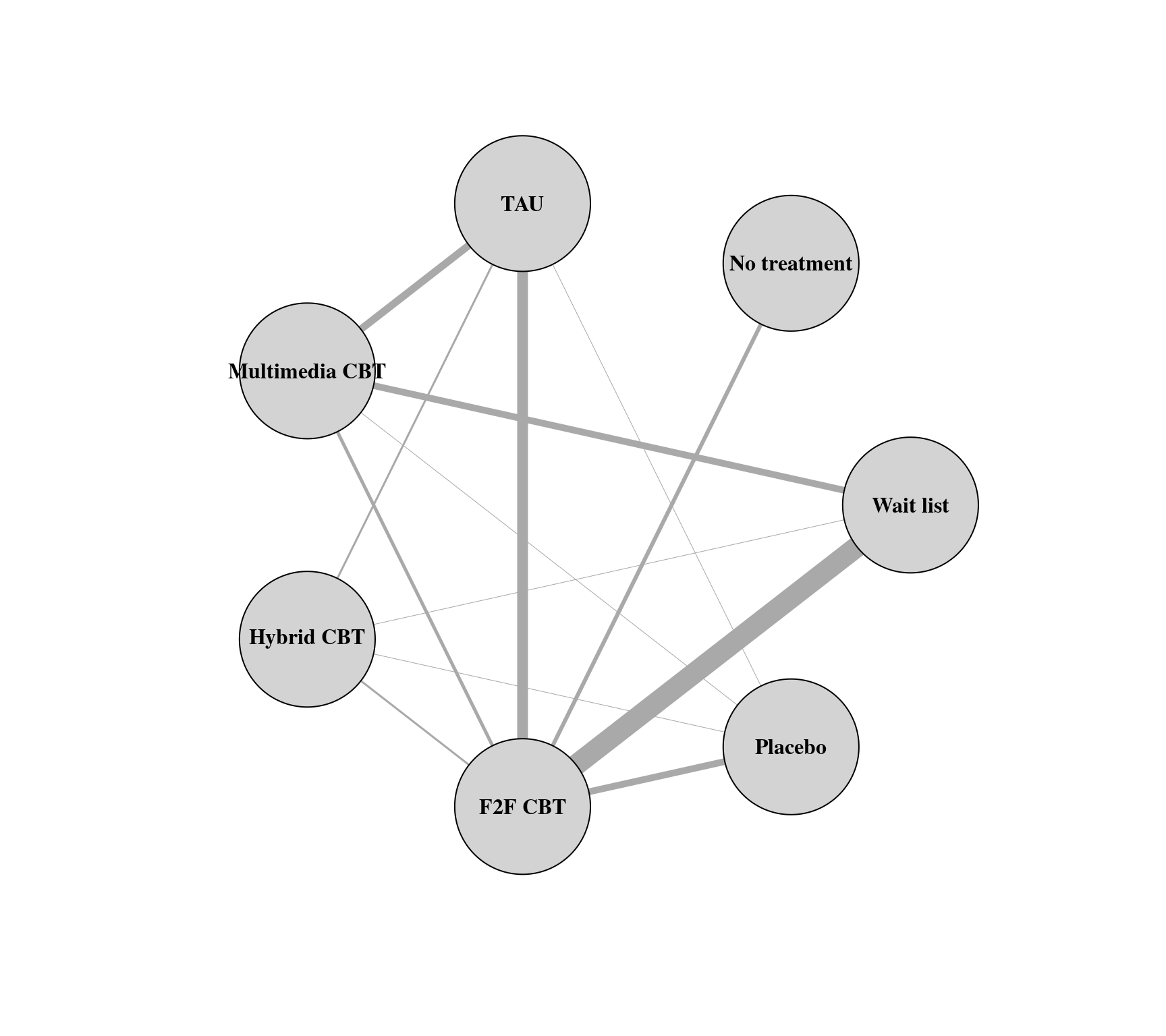
### create network graph ('igraph' package must be installed)
library(igraph, warn.conflicts=FALSE)
pairs <- data.frame(do.call(rbind,
sapply(split(dat$treatment, dat$study), function(x) t(combn(x,2)))), stringsAsFactors=FALSE)
pairs$X1 <- factor(pairs$X1, levels=sort(unique(dat$treatment)))
pairs$X2 <- factor(pairs$X2, levels=sort(unique(dat$treatment)))
tab <- table(pairs[,1], pairs[,2])
tab # adjacency matrix
#>
#> F2F CBT Hybrid CBT Multimedia CBT No treatment Placebo TAU Wait list
#> F2F CBT 17 3 5 0 0 0 0
#> Hybrid CBT 0 0 0 0 0 0 0
#> Multimedia CBT 0 0 5 0 0 0 0
#> No treatment 6 0 0 0 0 0 0
#> Placebo 10 1 1 0 0 0 0
#> TAU 16 3 11 0 1 0 0
#> Wait list 31 1 10 0 0 0 0
g <- graph_from_adjacency_matrix(tab, mode = "plus", weighted=TRUE, diag=FALSE)
plot(g, edge.curved=FALSE, edge.width=E(g)$weight/2,
layout=layout_in_circle(g, order=c("Wait list", "No treatment", "TAU", "Multimedia CBT",
"Hybrid CBT", "F2F CBT", "Placebo")),
vertex.size=45, vertex.color="lightgray", vertex.label.color="black", vertex.label.font=2)
 ### restructure data into wide format
dat <- to.wide(dat, study="study", grp="treatment", ref="TAU",
grpvars=c("diff","se","n"), postfix=c("1","2"))
### compute contrasts between treatment pairs and corresponding sampling variances
dat$yi <- with(dat, diff1 - diff2)
dat$vi <- with(dat, se1^2 + se2^2)
### calculate the variance-covariance matrix for multitreatment studies
calc.v <- function(x) {
v <- matrix(x$se2[1]^2, nrow=nrow(x), ncol=nrow(x))
diag(v) <- x$vi
v
}
V <- bldiag(lapply(split(dat, dat$study), calc.v))
### add contrast matrix to the dataset
dat <- contrmat(dat, grp1="treatment1", grp2="treatment2")
### network meta-analysis using a contrast-based random-effects model
### by setting rho=1/2, tau^2 reflects the amount of heterogeneity for all treatment comparisons
### the treatment left out (TAU) becomes the reference level for the treatment comparisons
res1 <- rma.mv(yi, V, data=dat,
mods = ~ 0 + No.treatment + Wait.list + Placebo + F2F.CBT + Hybrid.CBT + Multimedia.CBT,
random = ~ comp | study, rho=1/2)
res1
#>
#> Multivariate Meta-Analysis Model (k = 96; method: REML)
#>
#> Variance Components:
#>
#> outer factor: study (nlvls = 76)
#> inner factor: comp (nlvls = 14)
#>
#> estim sqrt fixed
#> tau^2 1.6262 1.2752 no
#> rho 0.5000 yes
#>
#> Test for Residual Heterogeneity:
#> QE(df = 90) = 18276.4524, p-val < .0001
#>
#> Test of Moderators (coefficients 1:6):
#> QM(df = 6) = 74.8404, p-val < .0001
#>
#> Model Results:
#>
#> estimate se zval pval ci.lb ci.ub
#> No.treatment 0.1975 0.5905 0.3344 0.7381 -0.9599 1.3548
#> Wait.list 0.7030 0.3471 2.0253 0.0428 0.0227 1.3834 *
#> Placebo -0.3699 0.4623 -0.8002 0.4236 -1.2760 0.5362
#> F2F.CBT -1.1177 0.2730 -4.0943 <.0001 -1.6527 -0.5826 ***
#> Hybrid.CBT -1.0781 0.5190 -2.0775 0.0378 -2.0953 -0.0610 *
#> Multimedia.CBT -0.6017 0.3399 -1.7700 0.0767 -1.2679 0.0646 .
#>
#> ---
#> Signif. codes: 0 ‘***’ 0.001 ‘**’ 0.01 ‘*’ 0.05 ‘.’ 0.1 ‘ ’ 1
#>
### forest plot of the contrast estimates (treatments versus TAU)
forest(coef(res1), diag(vcov(res1)), slab=sub(".", " ", names(coef(res1)), fixed=TRUE),
xlim=c(-5,5), alim=c(-3,3), psize=1, header="Treatment",
xlab="Difference in Standardized Mean Change (compared to TAU)")
### restructure data into wide format
dat <- to.wide(dat, study="study", grp="treatment", ref="TAU",
grpvars=c("diff","se","n"), postfix=c("1","2"))
### compute contrasts between treatment pairs and corresponding sampling variances
dat$yi <- with(dat, diff1 - diff2)
dat$vi <- with(dat, se1^2 + se2^2)
### calculate the variance-covariance matrix for multitreatment studies
calc.v <- function(x) {
v <- matrix(x$se2[1]^2, nrow=nrow(x), ncol=nrow(x))
diag(v) <- x$vi
v
}
V <- bldiag(lapply(split(dat, dat$study), calc.v))
### add contrast matrix to the dataset
dat <- contrmat(dat, grp1="treatment1", grp2="treatment2")
### network meta-analysis using a contrast-based random-effects model
### by setting rho=1/2, tau^2 reflects the amount of heterogeneity for all treatment comparisons
### the treatment left out (TAU) becomes the reference level for the treatment comparisons
res1 <- rma.mv(yi, V, data=dat,
mods = ~ 0 + No.treatment + Wait.list + Placebo + F2F.CBT + Hybrid.CBT + Multimedia.CBT,
random = ~ comp | study, rho=1/2)
res1
#>
#> Multivariate Meta-Analysis Model (k = 96; method: REML)
#>
#> Variance Components:
#>
#> outer factor: study (nlvls = 76)
#> inner factor: comp (nlvls = 14)
#>
#> estim sqrt fixed
#> tau^2 1.6262 1.2752 no
#> rho 0.5000 yes
#>
#> Test for Residual Heterogeneity:
#> QE(df = 90) = 18276.4524, p-val < .0001
#>
#> Test of Moderators (coefficients 1:6):
#> QM(df = 6) = 74.8404, p-val < .0001
#>
#> Model Results:
#>
#> estimate se zval pval ci.lb ci.ub
#> No.treatment 0.1975 0.5905 0.3344 0.7381 -0.9599 1.3548
#> Wait.list 0.7030 0.3471 2.0253 0.0428 0.0227 1.3834 *
#> Placebo -0.3699 0.4623 -0.8002 0.4236 -1.2760 0.5362
#> F2F.CBT -1.1177 0.2730 -4.0943 <.0001 -1.6527 -0.5826 ***
#> Hybrid.CBT -1.0781 0.5190 -2.0775 0.0378 -2.0953 -0.0610 *
#> Multimedia.CBT -0.6017 0.3399 -1.7700 0.0767 -1.2679 0.0646 .
#>
#> ---
#> Signif. codes: 0 ‘***’ 0.001 ‘**’ 0.01 ‘*’ 0.05 ‘.’ 0.1 ‘ ’ 1
#>
### forest plot of the contrast estimates (treatments versus TAU)
forest(coef(res1), diag(vcov(res1)), slab=sub(".", " ", names(coef(res1)), fixed=TRUE),
xlim=c(-5,5), alim=c(-3,3), psize=1, header="Treatment",
xlab="Difference in Standardized Mean Change (compared to TAU)")
 ### fit random inconsistency effects model (might have to switch optimizer to get convergence)
res2 <- rma.mv(yi, V, data=dat,
mods = ~ 0 + No.treatment + Wait.list + Placebo + F2F.CBT + Hybrid.CBT + Multimedia.CBT,
random = list(~ comp | study, ~ comp | design), rho=1/2, phi=1/2,
control=list(optimizer="BFGS"))
res2
#>
#> Multivariate Meta-Analysis Model (k = 96; method: REML)
#>
#> Variance Components:
#>
#> outer factor: study (nlvls = 76)
#> inner factor: comp (nlvls = 14)
#>
#> estim sqrt fixed
#> tau^2 1.6262 1.2752 no
#> rho 0.5000 yes
#>
#> outer factor: design (nlvls = 20)
#> inner factor: comp (nlvls = 14)
#>
#> estim sqrt fixed
#> gamma^2 0.0000 0.0054 no
#> phi 0.5000 yes
#>
#> Test for Residual Heterogeneity:
#> QE(df = 90) = 18276.4524, p-val < .0001
#>
#> Test of Moderators (coefficients 1:6):
#> QM(df = 6) = 74.8282, p-val < .0001
#>
#> Model Results:
#>
#> estimate se zval pval ci.lb ci.ub
#> No.treatment 0.1975 0.5905 0.3344 0.7380 -0.9599 1.3549
#> Wait.list 0.7030 0.3471 2.0252 0.0429 0.0226 1.3834 *
#> Placebo -0.3699 0.4623 -0.8000 0.4237 -1.2760 0.5362
#> F2F.CBT -1.1177 0.2730 -4.0938 <.0001 -1.6528 -0.5826 ***
#> Hybrid.CBT -1.0781 0.5190 -2.0774 0.0378 -2.0953 -0.0610 *
#> Multimedia.CBT -0.6017 0.3399 -1.7700 0.0767 -1.2680 0.0646 .
#>
#> ---
#> Signif. codes: 0 ‘***’ 0.001 ‘**’ 0.01 ‘*’ 0.05 ‘.’ 0.1 ‘ ’ 1
#>
### likelihood ratio test comparing the two models
anova(res1, res2)
#>
#> df AIC BIC AICc logLik LRT pval QE
#> Full 8 669.0347 689.0332 670.8125 -326.5174 18276.4524
#> Reduced 7 667.0344 684.5331 668.4003 -326.5172 0.0000 1.0000 18276.4524
#>
### collapse the different CBT forms into a single category
dat$CBT <- with(dat, ifelse(F2F.CBT + Hybrid.CBT + Multimedia.CBT > 0, 1, 0))
### fit the model with this treatment indicator
res3 <- rma.mv(yi, V, data=dat,
mods = ~ 0 + No.treatment + Wait.list + Placebo + CBT,
random = ~ comp | study, rho=1/2)
res3
#>
#> Multivariate Meta-Analysis Model (k = 96; method: REML)
#>
#> Variance Components:
#>
#> outer factor: study (nlvls = 76)
#> inner factor: comp (nlvls = 14)
#>
#> estim sqrt fixed
#> tau^2 1.6328 1.2778 no
#> rho 0.5000 yes
#>
#> Test for Residual Heterogeneity:
#> QE(df = 92) = 18501.2181, p-val < .0001
#>
#> Test of Moderators (coefficients 1:4):
#> QM(df = 4) = 72.1823, p-val < .0001
#>
#> Model Results:
#>
#> estimate se zval pval ci.lb ci.ub
#> No.treatment 0.3552 0.5792 0.6133 0.5397 -0.7800 1.4904
#> Wait.list 0.7190 0.3447 2.0862 0.0370 0.0435 1.3946 *
#> Placebo -0.2746 0.4584 -0.5992 0.5491 -1.1731 0.6238
#> CBT -0.9599 0.2454 -3.9117 <.0001 -1.4409 -0.4790 ***
#>
#> ---
#> Signif. codes: 0 ‘***’ 0.001 ‘**’ 0.01 ‘*’ 0.05 ‘.’ 0.1 ‘ ’ 1
#>
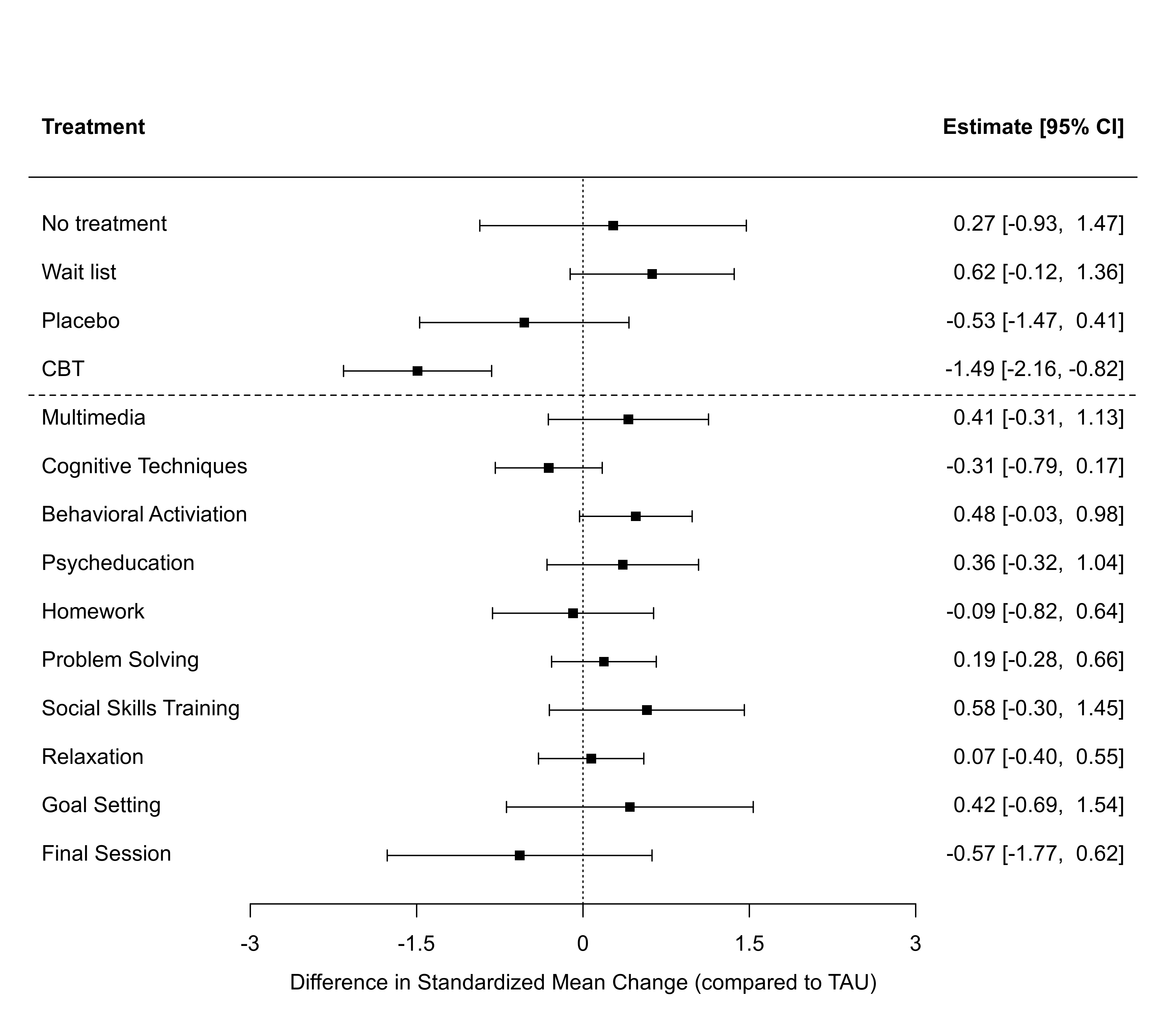
### component network meta-analysis (effect of CBT may be larger/smaller depending on
### the presence of various components; leaving out 'mind' and 'act' as in the paper)
res4 <- rma.mv(yi, V, data=dat,
mods = ~ 0 + No.treatment + Wait.list + Placebo + CBT +
CBT:(multi + cog + ba + psed + home + prob + soc + relax + goal + final),
random = ~ comp | study, rho=1/2)
res4
#>
#> Multivariate Meta-Analysis Model (k = 96; method: REML)
#>
#> Variance Components:
#>
#> outer factor: study (nlvls = 76)
#> inner factor: comp (nlvls = 14)
#>
#> estim sqrt fixed
#> tau^2 1.6107 1.2691 no
#> rho 0.5000 yes
#>
#> Test for Residual Heterogeneity:
#> QE(df = 82) = 12774.6232, p-val < .0001
#>
#> Test of Moderators (coefficients 1:14):
#> QM(df = 14) = 247.2504, p-val < .0001
#>
#> Model Results:
#>
#> estimate se zval pval ci.lb ci.ub
#> No.treatment 0.2712 0.6131 0.4424 0.6582 -0.9304 1.4729
#> Wait.list 0.6238 0.3774 1.6531 0.0983 -0.1158 1.3635 .
#> Placebo -0.5293 0.4815 -1.0992 0.2717 -1.4730 0.4145
#> CBT -1.4915 0.3407 -4.3778 <.0001 -2.1593 -0.8237 ***
#> CBT:multi 0.4097 0.3685 1.1118 0.2662 -0.3125 1.1319
#> CBT:cog -0.3086 0.2460 -1.2546 0.2096 -0.7908 0.1735
#> CBT:ba 0.4766 0.2590 1.8401 0.0658 -0.0310 0.9843 .
#> CBT:psed 0.3588 0.3486 1.0293 0.3034 -0.3244 1.0420
#> CBT:home -0.0896 0.3705 -0.2419 0.8089 -0.8158 0.6366
#> CBT:prob 0.1888 0.2408 0.7840 0.4330 -0.2832 0.6608
#> CBT:soc 0.5758 0.4485 1.2837 0.1992 -0.3033 1.4549
#> CBT:relax 0.0735 0.2422 0.3035 0.7615 -0.4013 0.5483
#> CBT:goal 0.4226 0.5676 0.7446 0.4565 -0.6899 1.5351
#> CBT:final -0.5714 0.6091 -0.9381 0.3482 -1.7653 0.6224
#>
#> ---
#> Signif. codes: 0 ‘***’ 0.001 ‘**’ 0.01 ‘*’ 0.05 ‘.’ 0.1 ‘ ’ 1
#>
rownames <- names(coef(res4))
rownames <- sub(".", " ", rownames, fixed=TRUE)
rownames[5:14] <- c("Multimedia", "Cognitive Techniques", "Behavioral Activiation",
"Psycheducation", "Homework", "Problem Solving", "Social Skills Training",
"Relaxation", "Goal Setting", "Final Session")
### forest plot of the estimates
forest(coef(res4), diag(vcov(res4)), slab=rownames,
xlim=c(-5,5), alim=c(-3,3), psize=1, header="Treatment",
xlab="Difference in Standardized Mean Change (compared to TAU)")
abline(h=10.5, lty="dashed")
### fit random inconsistency effects model (might have to switch optimizer to get convergence)
res2 <- rma.mv(yi, V, data=dat,
mods = ~ 0 + No.treatment + Wait.list + Placebo + F2F.CBT + Hybrid.CBT + Multimedia.CBT,
random = list(~ comp | study, ~ comp | design), rho=1/2, phi=1/2,
control=list(optimizer="BFGS"))
res2
#>
#> Multivariate Meta-Analysis Model (k = 96; method: REML)
#>
#> Variance Components:
#>
#> outer factor: study (nlvls = 76)
#> inner factor: comp (nlvls = 14)
#>
#> estim sqrt fixed
#> tau^2 1.6262 1.2752 no
#> rho 0.5000 yes
#>
#> outer factor: design (nlvls = 20)
#> inner factor: comp (nlvls = 14)
#>
#> estim sqrt fixed
#> gamma^2 0.0000 0.0054 no
#> phi 0.5000 yes
#>
#> Test for Residual Heterogeneity:
#> QE(df = 90) = 18276.4524, p-val < .0001
#>
#> Test of Moderators (coefficients 1:6):
#> QM(df = 6) = 74.8282, p-val < .0001
#>
#> Model Results:
#>
#> estimate se zval pval ci.lb ci.ub
#> No.treatment 0.1975 0.5905 0.3344 0.7380 -0.9599 1.3549
#> Wait.list 0.7030 0.3471 2.0252 0.0429 0.0226 1.3834 *
#> Placebo -0.3699 0.4623 -0.8000 0.4237 -1.2760 0.5362
#> F2F.CBT -1.1177 0.2730 -4.0938 <.0001 -1.6528 -0.5826 ***
#> Hybrid.CBT -1.0781 0.5190 -2.0774 0.0378 -2.0953 -0.0610 *
#> Multimedia.CBT -0.6017 0.3399 -1.7700 0.0767 -1.2680 0.0646 .
#>
#> ---
#> Signif. codes: 0 ‘***’ 0.001 ‘**’ 0.01 ‘*’ 0.05 ‘.’ 0.1 ‘ ’ 1
#>
### likelihood ratio test comparing the two models
anova(res1, res2)
#>
#> df AIC BIC AICc logLik LRT pval QE
#> Full 8 669.0347 689.0332 670.8125 -326.5174 18276.4524
#> Reduced 7 667.0344 684.5331 668.4003 -326.5172 0.0000 1.0000 18276.4524
#>
### collapse the different CBT forms into a single category
dat$CBT <- with(dat, ifelse(F2F.CBT + Hybrid.CBT + Multimedia.CBT > 0, 1, 0))
### fit the model with this treatment indicator
res3 <- rma.mv(yi, V, data=dat,
mods = ~ 0 + No.treatment + Wait.list + Placebo + CBT,
random = ~ comp | study, rho=1/2)
res3
#>
#> Multivariate Meta-Analysis Model (k = 96; method: REML)
#>
#> Variance Components:
#>
#> outer factor: study (nlvls = 76)
#> inner factor: comp (nlvls = 14)
#>
#> estim sqrt fixed
#> tau^2 1.6328 1.2778 no
#> rho 0.5000 yes
#>
#> Test for Residual Heterogeneity:
#> QE(df = 92) = 18501.2181, p-val < .0001
#>
#> Test of Moderators (coefficients 1:4):
#> QM(df = 4) = 72.1823, p-val < .0001
#>
#> Model Results:
#>
#> estimate se zval pval ci.lb ci.ub
#> No.treatment 0.3552 0.5792 0.6133 0.5397 -0.7800 1.4904
#> Wait.list 0.7190 0.3447 2.0862 0.0370 0.0435 1.3946 *
#> Placebo -0.2746 0.4584 -0.5992 0.5491 -1.1731 0.6238
#> CBT -0.9599 0.2454 -3.9117 <.0001 -1.4409 -0.4790 ***
#>
#> ---
#> Signif. codes: 0 ‘***’ 0.001 ‘**’ 0.01 ‘*’ 0.05 ‘.’ 0.1 ‘ ’ 1
#>
### component network meta-analysis (effect of CBT may be larger/smaller depending on
### the presence of various components; leaving out 'mind' and 'act' as in the paper)
res4 <- rma.mv(yi, V, data=dat,
mods = ~ 0 + No.treatment + Wait.list + Placebo + CBT +
CBT:(multi + cog + ba + psed + home + prob + soc + relax + goal + final),
random = ~ comp | study, rho=1/2)
res4
#>
#> Multivariate Meta-Analysis Model (k = 96; method: REML)
#>
#> Variance Components:
#>
#> outer factor: study (nlvls = 76)
#> inner factor: comp (nlvls = 14)
#>
#> estim sqrt fixed
#> tau^2 1.6107 1.2691 no
#> rho 0.5000 yes
#>
#> Test for Residual Heterogeneity:
#> QE(df = 82) = 12774.6232, p-val < .0001
#>
#> Test of Moderators (coefficients 1:14):
#> QM(df = 14) = 247.2504, p-val < .0001
#>
#> Model Results:
#>
#> estimate se zval pval ci.lb ci.ub
#> No.treatment 0.2712 0.6131 0.4424 0.6582 -0.9304 1.4729
#> Wait.list 0.6238 0.3774 1.6531 0.0983 -0.1158 1.3635 .
#> Placebo -0.5293 0.4815 -1.0992 0.2717 -1.4730 0.4145
#> CBT -1.4915 0.3407 -4.3778 <.0001 -2.1593 -0.8237 ***
#> CBT:multi 0.4097 0.3685 1.1118 0.2662 -0.3125 1.1319
#> CBT:cog -0.3086 0.2460 -1.2546 0.2096 -0.7908 0.1735
#> CBT:ba 0.4766 0.2590 1.8401 0.0658 -0.0310 0.9843 .
#> CBT:psed 0.3588 0.3486 1.0293 0.3034 -0.3244 1.0420
#> CBT:home -0.0896 0.3705 -0.2419 0.8089 -0.8158 0.6366
#> CBT:prob 0.1888 0.2408 0.7840 0.4330 -0.2832 0.6608
#> CBT:soc 0.5758 0.4485 1.2837 0.1992 -0.3033 1.4549
#> CBT:relax 0.0735 0.2422 0.3035 0.7615 -0.4013 0.5483
#> CBT:goal 0.4226 0.5676 0.7446 0.4565 -0.6899 1.5351
#> CBT:final -0.5714 0.6091 -0.9381 0.3482 -1.7653 0.6224
#>
#> ---
#> Signif. codes: 0 ‘***’ 0.001 ‘**’ 0.01 ‘*’ 0.05 ‘.’ 0.1 ‘ ’ 1
#>
rownames <- names(coef(res4))
rownames <- sub(".", " ", rownames, fixed=TRUE)
rownames[5:14] <- c("Multimedia", "Cognitive Techniques", "Behavioral Activiation",
"Psycheducation", "Homework", "Problem Solving", "Social Skills Training",
"Relaxation", "Goal Setting", "Final Session")
### forest plot of the estimates
forest(coef(res4), diag(vcov(res4)), slab=rownames,
xlim=c(-5,5), alim=c(-3,3), psize=1, header="Treatment",
xlab="Difference in Standardized Mean Change (compared to TAU)")
abline(h=10.5, lty="dashed")